Machine Learning Research: Cost-Aware Tracker Blocking in Firefox: Index
Firefox serves more than 200 million users worldwide, each blocking thousands of tracker requests per month. Enhanced Tracking Protection, Firefox’s built-in tracker blocker, was a silent feature: blocks happened in the background and were never surfaced. Over Fall 2025 and Winter 2026, the Mozilla Privacy team built a new-tab privacy widget to give users visibility into ETP. I shipped the widget itself (the UI component, the metrics service, the aggregation pipeline) and watched it land as a count: “147 trackers blocked this week.”
The count was honest but uninformative. A single-pixel beacon counts the same as a 170 KB JavaScript SDK. Two users who both see “147 blocked” may have had wildly different amounts of bandwidth, CPU, and time saved. The widget was a privacy product reporting a privacy metric, but the user-facing number didn’t reflect the size of the privacy intervention.
This project closes that gap. We built a model that converts each block into a cost estimate (bytes that would have crossed the wire, milliseconds of download time avoided) and integrated it into the widget I had already shipped. The model is a 500 KB ONNX artifact alongside the existing blocklist, runs in ~50 µs on the device, and predicts the cost of something that, by design, never happened.
This page is the canonical write-up. The four linked articles at the bottom go deeper on data, modeling, learned representations, and deployment.
The problem
Enhanced Tracking Protection blocks third-party requests identified by the Disconnect list, a public set of tracker domains maintained by Disconnect.me. The block fires before the network request is issued, which is the privacy property that matters: no data leaves the device. As a side effect, the response never arrives. The browser observes the request URL, resource type, initiator, and HTTP metadata, then drops the request. It never sees how many bytes the server would have returned or how long the download would have taken.
The widget I shipped first reports counts because counts are the only quantity the browser directly observes. The cost, the thing the user actually cares about, is structurally unobservable. To report it, we have to predict it.
Three audiences need the cost answer. Users need it to understand what the browser is doing for them, beyond a number that mostly tracks how many ads a site tried to load. Blocklist maintainers need it to triage which Disconnect rules carry weight: a rule that blocks ten 200-byte pixels matters less than one that blocks a single 200 KB SDK. Privacy researchers need it to compare Firefox’s ETP to Brave Shields, Safari ITP, and uBlock Origin on something other than block counts, which any of them can game by adding more rules.
Why the problem is hard
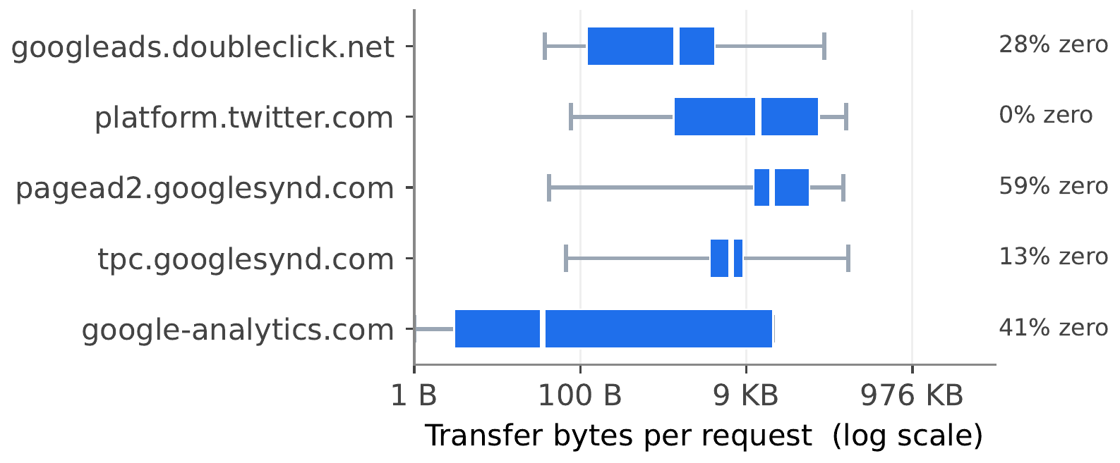
The natural baseline is to assign each tracker domain a static cost score. Aggregate every historical request for googletagmanager.com, compute the median transfer size, and use that whenever Firefox blocks a request to that domain. This is what most prior work does at the page level, and it fails for a structural reason: the URL path, not the domain, is the primary determinant of cost.
googletagmanager.com/gtag/js returns a 93 KB JavaScript bundle. googletagmanager.com/collect returns zero bytes. Same domain, three orders of magnitude apart. We measured this across all 3,723 tracker domains in our dataset and found a within-domain coefficient of variation of 0.94 at the median domain and 3.0 at the 90th percentile. Domain-level estimates collapse this variance into a single number, and any single number is wrong for most requests under that domain.
Adding resource type to the lookup key helps but not enough. A lookup table indexed by (domain, resource_type) brings test-set MAE down from 9,008 bytes to 6,802. Adding the exact URL path drops it to 4,326 bytes, but this approach is a trap for two reasons. First, the table grows to roughly 187 MB at full Firefox deployment scale, 350× the size of the model and far beyond what ships in Remote Settings. Second, a large fraction of unique URL paths in any given test set are unseen in training, because tracker SDKs continuously version their endpoints, embed campaign IDs in URLs, and shift their path structures. A path-level lookup table is both too large to ship and obsolete the day after it is built.
What is needed is a model that generalizes from URL structure rather than memorizing specific paths. A 93 KB JavaScript bundle and a zero-byte beacon look different in their URL tokens even when the model has never seen the exact path before. A learned representation can pick up on /gtag/js looking like a bundle and /collect looking like a beacon, and produce a sensible estimate either way.
Brave already shipped something. Here is why ours is different.
Brave shipped a bandwidth savings predictor in 2019. They report page-level estimates of how much data ad-blocking saved. Their approach uses paired crawls: load each page twice, once with blocking and once without, and use the difference in transferred bytes as the training label. The model is a linear regression that predicts the page-level total from page-level features. They report for bandwidth.
This is a different problem from ours in three ways. First, paired crawls are expensive to refresh: every training row requires loading the same page twice. Second, page-level prediction cannot attribute cost to individual trackers, so it cannot answer the blocklist-maintenance question of which rules pull weight. Third, translates to median session-level error around 2.7 MB, which is acceptable for a marketing number and insufficient for an accurate widget.
The contribution of our work is per-request prediction trained on completed responses, with no paired crawl required. The training population is HTTP Archive’s crawl of millions of pages, in which every request reaches completion and the response size is recorded. The deployment population is Firefox’s blocked requests, which never complete. The same URL returns the same number of bytes regardless of which browser issued the request, so the labels learned from HTTP Archive transfer cleanly to Firefox at inference time. This is a covariate shift problem, not a domain adaptation problem, and the conditional distribution is invariant by construction.
Crucially, we don’t just assert that the labels transfer — we measured it. The training crawl is Chrome-based and the model deploys into Firefox, so we ran a paired Firefox/Chrome fetch of 46 representative tracker URLs and quantified per-URL byte agreement at the request level: the median byte ratio is 1.000, and 97.8% of URLs agree within 5%. The single outlier is Google reCAPTCHA at 0.63, documented rather than hidden. The cross-browser assumption the whole project rests on is the assumption we tested most directly. (Details in Firefox ONNX inference.)
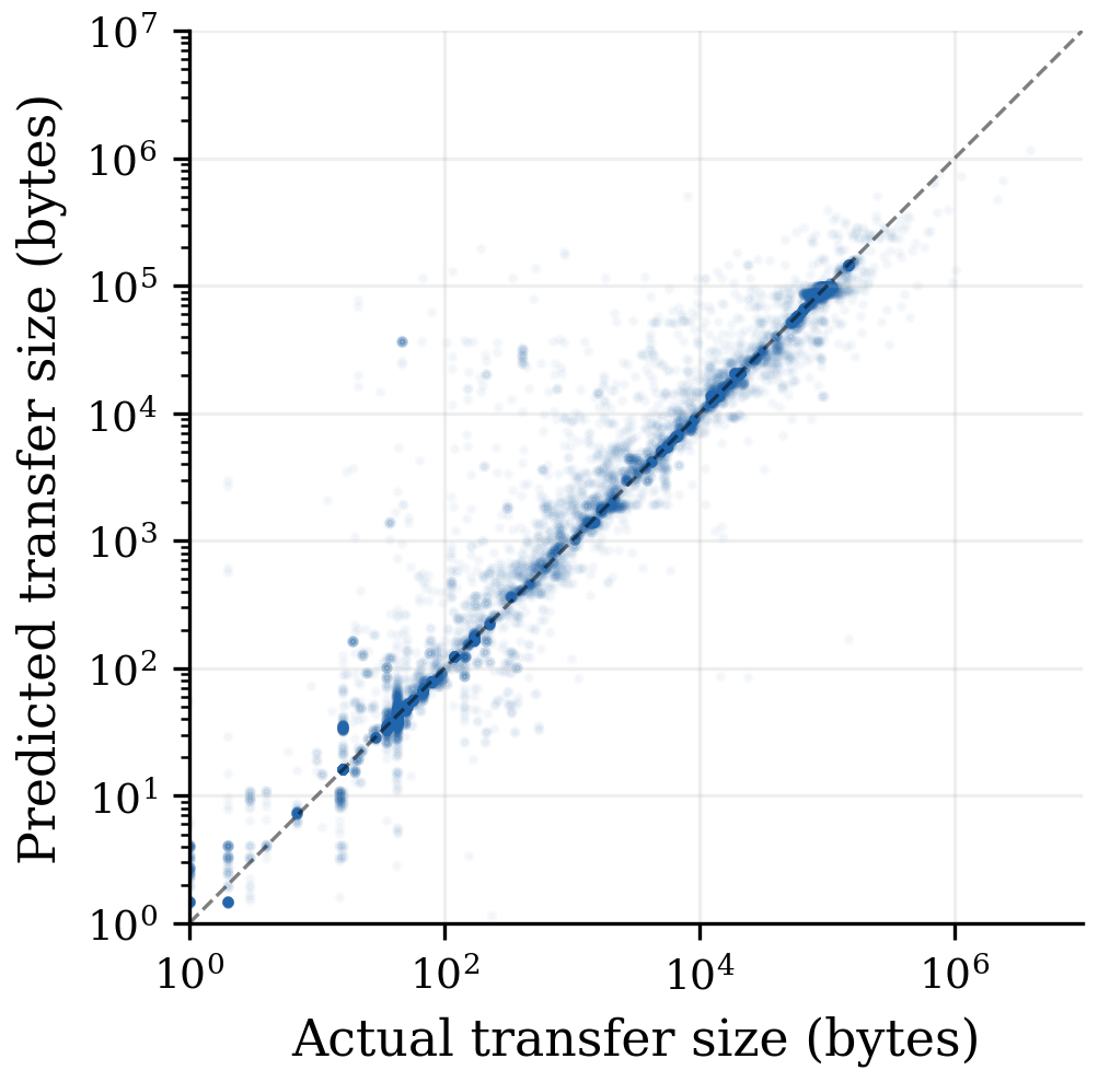
A linear model is not an option here, which is worth stating because Brave’s was linear. A Brave-style Ridge regression on our per-request features reaches MAE 9,651 — worse than the lookup table it would replace (6,802). Least-squares on a target with mean 13 KB and max 14 MB is swamped by the heavy right tail. The problem needs a loss matched to the distribution, which is the subject below.
Data
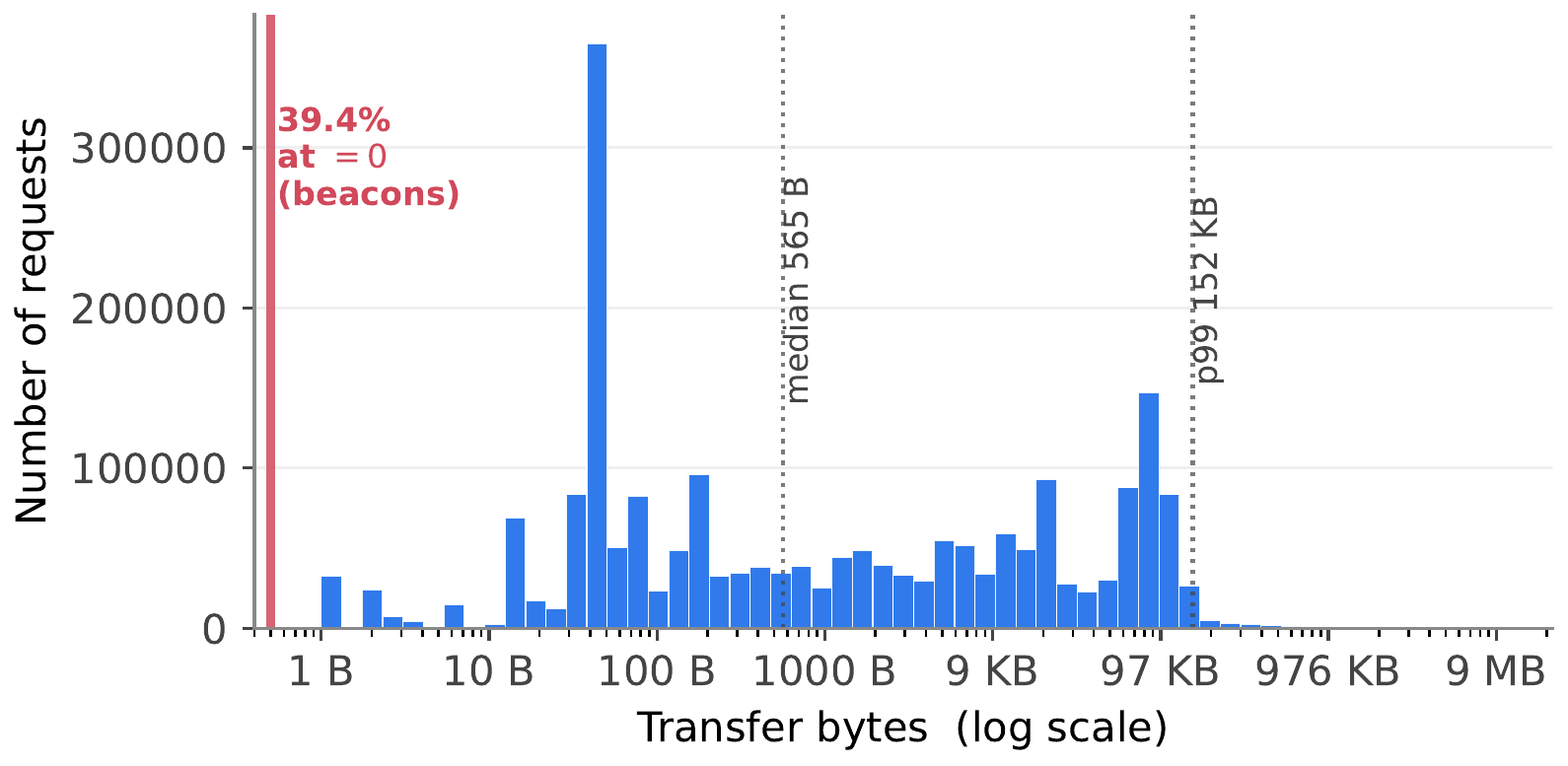
We use the HTTP Archive June 2024 mobile crawl, filtered to third-party requests in five Disconnect categories: advertising, analytics, social, tag-manager, and consent-provider. We sample deterministically via hash bucketing on (page, url), yielding 3,490,824 requests across 3,723 tracker domains, covering 92.5% of requests and 98.6% of bytes in the trained categories. Deterministic sampling makes the dataset reproducible.
The target is transfer_bytes: on-wire response size including headers. The distribution has two defining properties. 39.5% of requests return exactly zero bytes — tracking beacons that fire and forget. The remainder is a heavy-tailed positive distribution spanning four orders of magnitude, with a secondary mode near 90 KB (JavaScript SDK bundles). Median is 43 bytes, mean is 13,607 bytes, maximum is 14 MB.
This zero-inflated, heavy-tailed shape determines the loss function. Squared-error regression assumes the target is roughly Gaussian. Tracker responses are not. A loss that handles spike-at-zero and a long tail in a single objective is the dominant modeling choice in this project, and we return to it below.
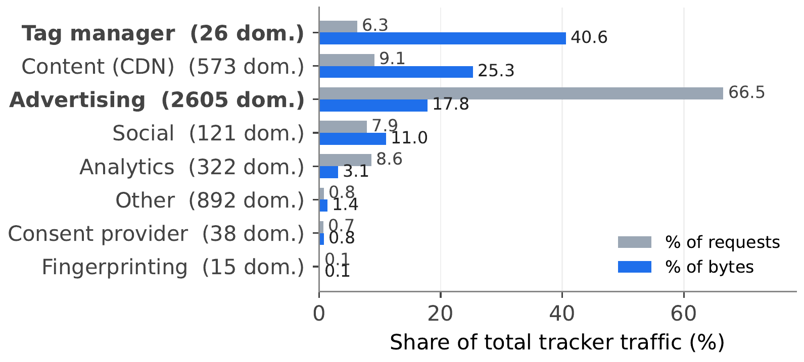
Before estimating the unobservable, it is worth measuring what is observable — the cost landscape ETP acts on. Blocked traffic is sharply concentrated: a 26-domain tag-manager category carries 41% of all blocked bytes from just 6% of requests, while advertising is 66.5% of requests but only 17.8% of bytes. A privacy product that only counts blocks treats the 200-byte advertising pixel and the 90 KB tag-manager bundle identically. The byte distribution is where the real intervention lives, which is exactly what the cost model is built to surface.
The 85-dimensional feature set falls into five groups, all observable from Firefox’s network stack at block time: domain target-encoding (median transfer_bytes per domain and per (domain, resource_type)); URL content (TF-IDF embeddings of path tokens reduced to 50 dimensions via truncated SVD); URL structure (path depth, length, query-parameter count, file extension); request metadata (resource type, initiator type, HTTP method, from nsILoadInfo); and a small set of hand-curated URL-pattern regex flags. The split is a random row split, which matches deployment: Firefox has training statistics for all Disconnect-list domains at inference time, so domain identity is a known feature.
The model
We train XGBoost with Tweedie loss. Hyperparameters: 500 trees, max depth 8, learning rate 0.05, early stopping on the validation set. The Tweedie variance power .
The architecture is the smallest thing that works. Tree-based gradient boosting is the standard choice for tabular regression at this scale, and the deployment constraint of a 500 KB ONNX artifact rules out neural architectures with embedding tables in the millions of parameters. Grinsztajn et al. (2022) document that tree-based models are competitive with or dominant over deep learning on tabular data below roughly 10K samples, with the gap narrowing at larger scales. At our scale a well-tuned XGBoost model produces accuracy that justifies the deployment cost.
The interesting modeling choice is not the architecture. It is the loss.
Tweedie loss, borrowed from actuarial science
Tracker response sizes have the same distributional shape as insurance claims. Most filings result in no claim (zero payout). The rest are heavy-tailed: a small number of catastrophic claims dominate the total payout. Actuarial scientists solved this in the 1980s with the Tweedie family of compound Poisson-Gamma distributions, which handles the zero mass and the heavy tail in a single likelihood.
The Tweedie loss with variance power is:
The gradient is weighted by predicted magnitude. Errors on near-zero predictions are penalized lightly; errors on large predictions are penalized heavily. This is exactly the right inductive bias for tracker cost prediction, where a small absolute error on a 200-byte beacon contributes nothing to the weekly bandwidth aggregate, while the same absolute error on a 90 KB script materially distorts the user-facing number.
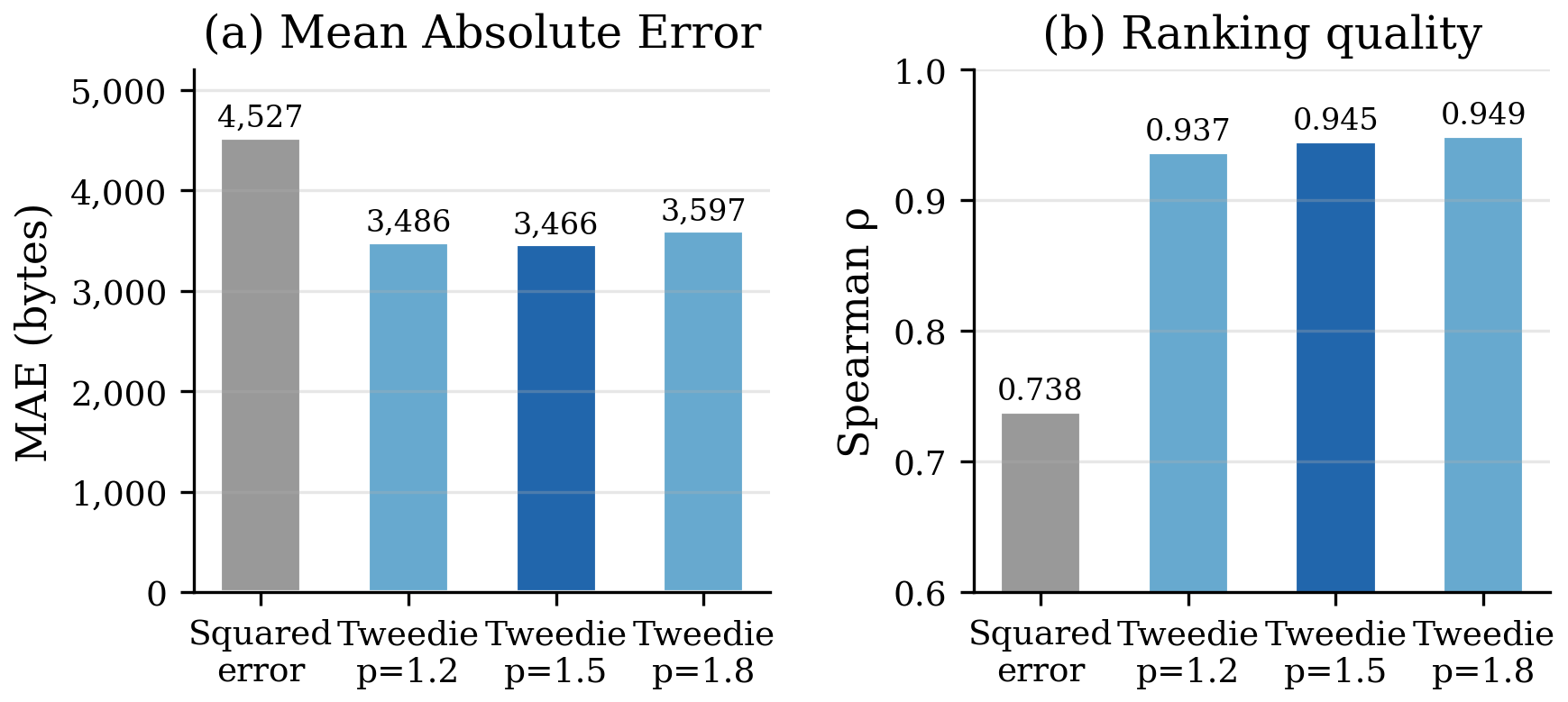
We confirmed this in ablation. Holding architecture and features constant, swapping squared-error loss for Tweedie loss reduces MAE by roughly 23%. The Tweedie variance power is robust: the ~4% sensitivity to across is dwarfed by the 23% gap from switching losses. The loss is the dominant modeling choice; the power parameter is a rounding error by comparison.
The methodological transfer is the contribution. The result is not “we trained an XGBoost on tabular data.” It is “the right loss function for this data shape was sitting in another field, and applying it produces a larger gain than any architecture or feature-engineering decision we made.” For zero-inflated web measurement data more broadly, this generalizes: loss-function selection dominates.
Results
On the held-out test split, plotted against artifact size (the deployment constraint):
| Approach | Size | MAE (bytes) | 95% CI |
|---|---|---|---|
| Global median | <1 B | 19,905 | --- |
| Domain LUT | 88 KB | 9,008 | --- |
| Domain + type LUT (deployed) | 114 KB | 6,802 | [6,633, 6,977] |
| Path LUT (not deployable) | 187 MB | 4,326 | [4,154, 4,516] |
| XGBoost Tweedie | 500 KB | 4,246 | [4,079, 4,442] |
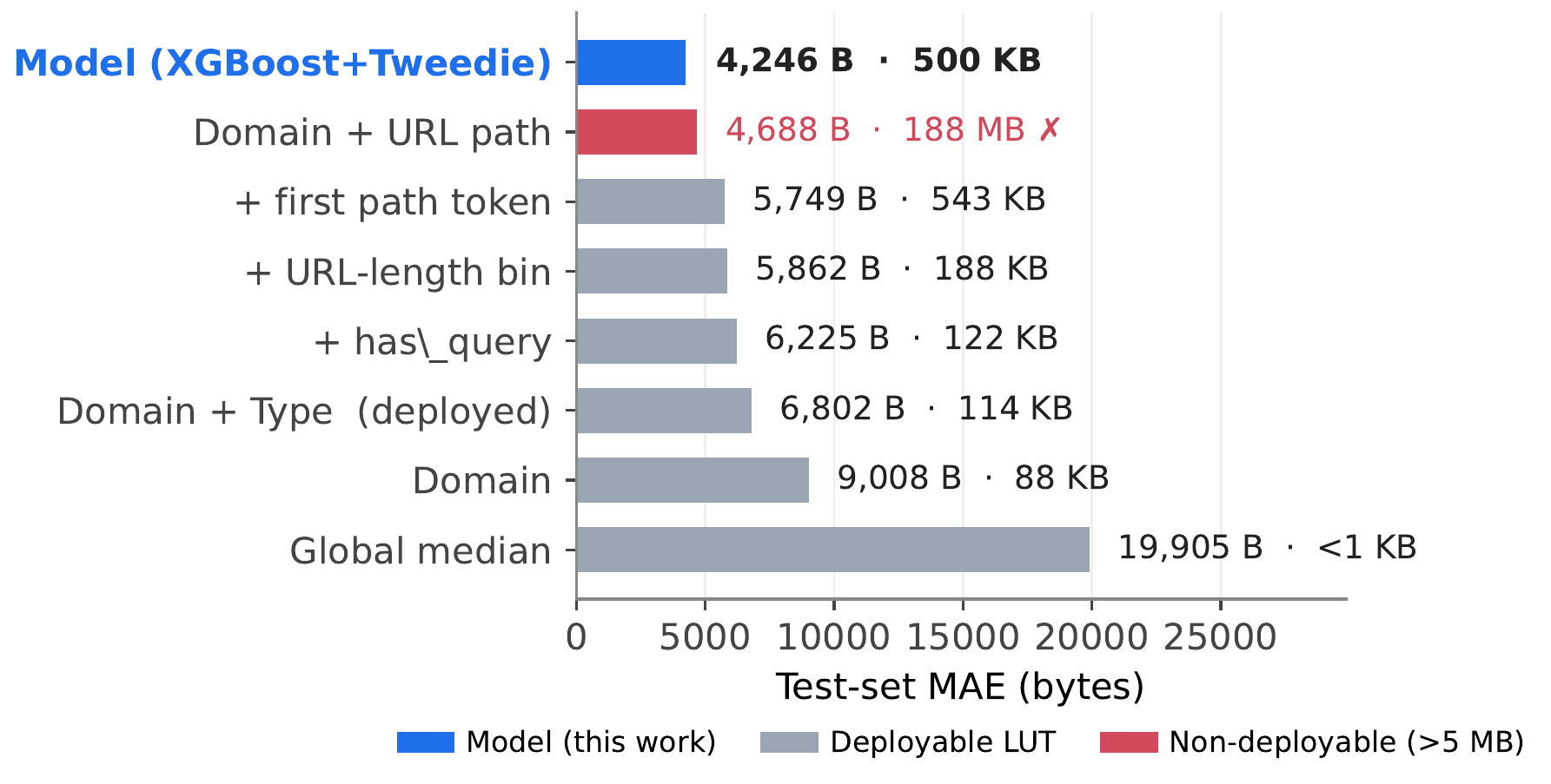
The headline is a 37.6% MAE reduction over the deployed domain+type lookup table. But the sharper story is the comparison against the path-level table: that table reaches essentially the same accuracy as the model (4,326 vs 4,246) — and weighs 187 MB at deployment scale, 350× the size of the model. The model is the only point in the lookup-table ladder that achieves URL-level accuracy at a size that ships in Remote Settings. ML earns its place here not by being the most accurate thing possible, but by being the most accurate thing that fits.
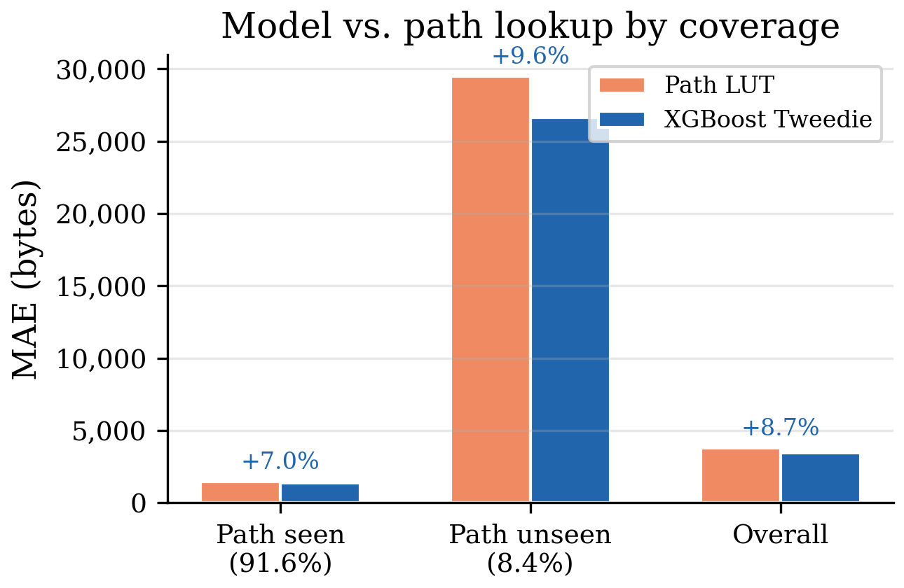
Decomposing by path coverage is the cleanest test of generalization-vs-memorization. On the ~92% of test rows the path LUT can serve, it has the exact answer memorized — and the model matches it (model 2,264 vs LUT 1,811 bytes), coming up slightly behind per-request, which is exactly what you’d expect: the LUT looked up the training median, the model generalized. But it matches that at 350× smaller size, and with lower systematic bias, which is what matters once you aggregate. On the ~8% of rows with unseen paths — disproportionately expensive — the model clearly wins (27,224 vs 33,471), generalizing from URL structure where the table can only fall back to a coarse aggregate.
The honest framing: the model does not beat a memorized lookup table on its home turf. It ties it there at a fraction of the size, and pulls ahead exactly where memorization breaks (unseen paths) and where the user reads the number (aggregation). We ruled out the simpler explanation that Laplace smoothing of the path LUT would close the gap — it does not. The model’s edge is a learned cross-path representation, not a regularization trick a table could copy.
What the user sees: weekly aggregation
Users do not see per-request predictions. They see weekly totals on the new-tab page: the widget I built, now annotated with cost instead of just count. “Firefox saved you 2.3 MB this week.” The relevant accuracy is therefore the error on the sum of predictions, not the error on any individual prediction.
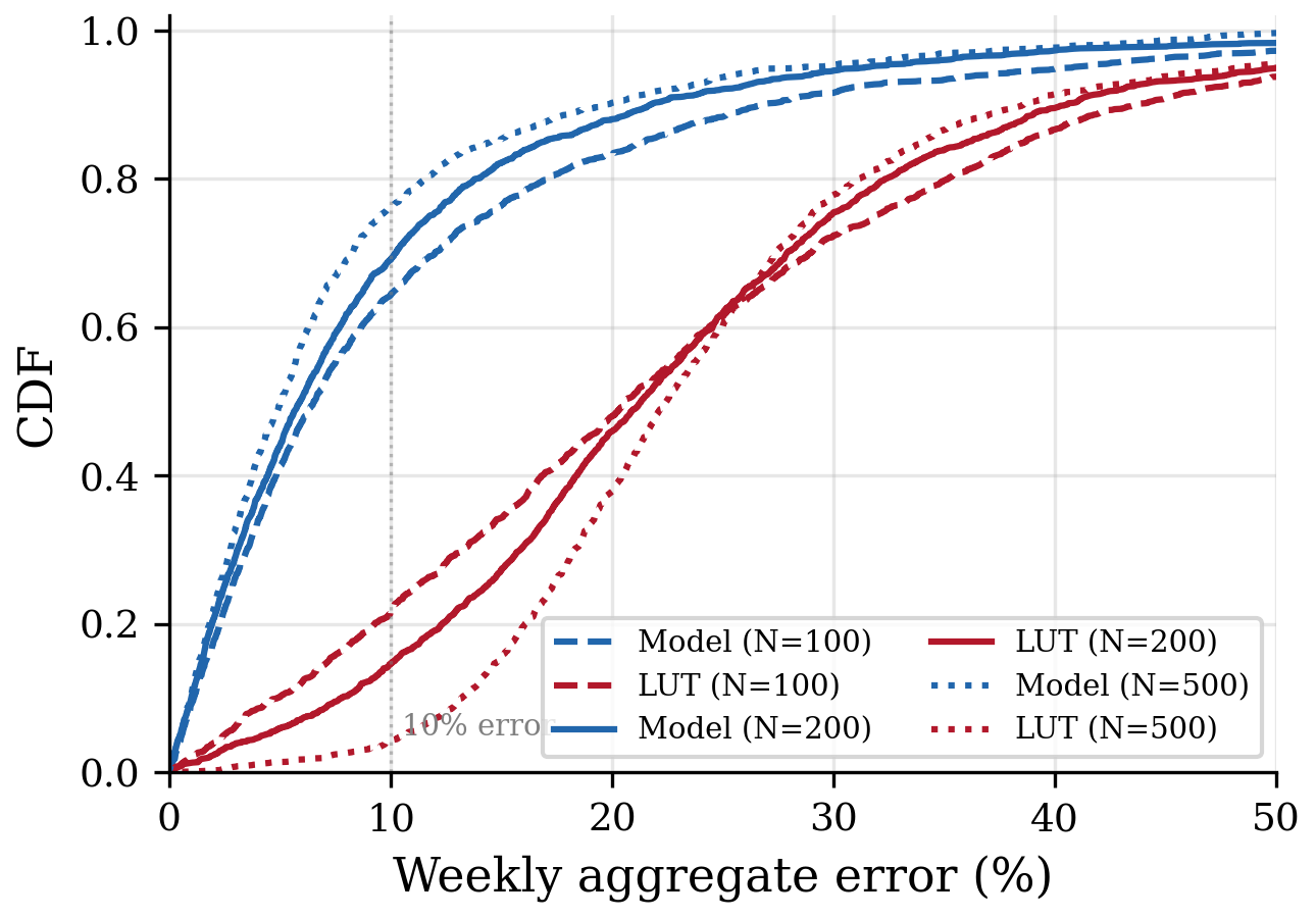
This matters because the model’s per-request error is not the user-facing error. We simulate weekly browsing by sampling blocked requests with replacement from the test set, summing predicted and true transfer sizes, and computing percentage error. Repeated 2,000 times to get a distribution.
At blocked requests per week, the model’s median weekly error is 6.0%, while the deployed domain+type lookup table sits at 21.9%. The gap widens with more requests: at , the model improves to 5.1% median error while the LUT degrades to 23.2%.
The reason the LUT degrades is that its errors are systematic. The constant per-bucket median consistently underpredicts script sizes and overpredicts beacon costs, and those biases compound in the sum. The model’s errors are approximately mean-zero across the distribution and cancel under aggregation. Per-request noise is not the same kind of error as per-request bias, and aggregation is the operation that makes the difference visible.
This finding extends to targets where the model is worse than the LUT per-request. We also predicted download duration, time-to-first-byte, and total page load time. On TTFB and load time, per-request MAE was slightly worse than the LUT, because timing is network- and device-dependent and the URL features do not predict it well. But in weekly aggregation, the model still beats the LUT on all four targets, because the LUT’s systematic bias compounds regardless of the metric. Per-request accuracy and aggregate accuracy are different objectives, and the user-facing one rewards low bias far more than low noise.
Robustness checks
The uniform aggregation simulation is unrealistic in one direction: real users do not visit a uniform random sample of pages. They return to a small set of sites repeatedly, which means blocked requests cluster on a small set of tracker domains. We re-ran the simulation with domain-correlated sampling (sample 15 domains per simulated week, then draw requests only from those) to test whether the model’s advantage survives.
At , domain-correlated browsing roughly doubles the model’s median error from 6.0% to 12.9%. The LUT’s error rises further, from 21.9% to 36.4%. The model’s advantage widens under correlation, because the LUT’s per-domain bias compounds more severely when browsing concentrates on fewer domains, while the model retains within-domain discriminative signal from URL features. The realistic browsing pattern is the one where the model helps most.
We also tested temporal generalization directly (covered in full in the “Robustness across time” section above): evaluated on crawls 1, 3, and 6 months out, the model holds a per-request advantage of +33.5% / +28.9% / +25.6% over the lookup table, and a user-facing aggregation advantage that erodes only from +13 pp to +5.7 pp. URL path churn in versioned script bundles, not domain churn, drives the decay. The 3-month aggregation gap of +10.8 pp is what sets the quarterly retraining cadence.
The implication for deployment is a quarterly retraining cadence on fresh HTTP Archive crawls, which is feasible given the monthly crawl release schedule.
Robustness across time
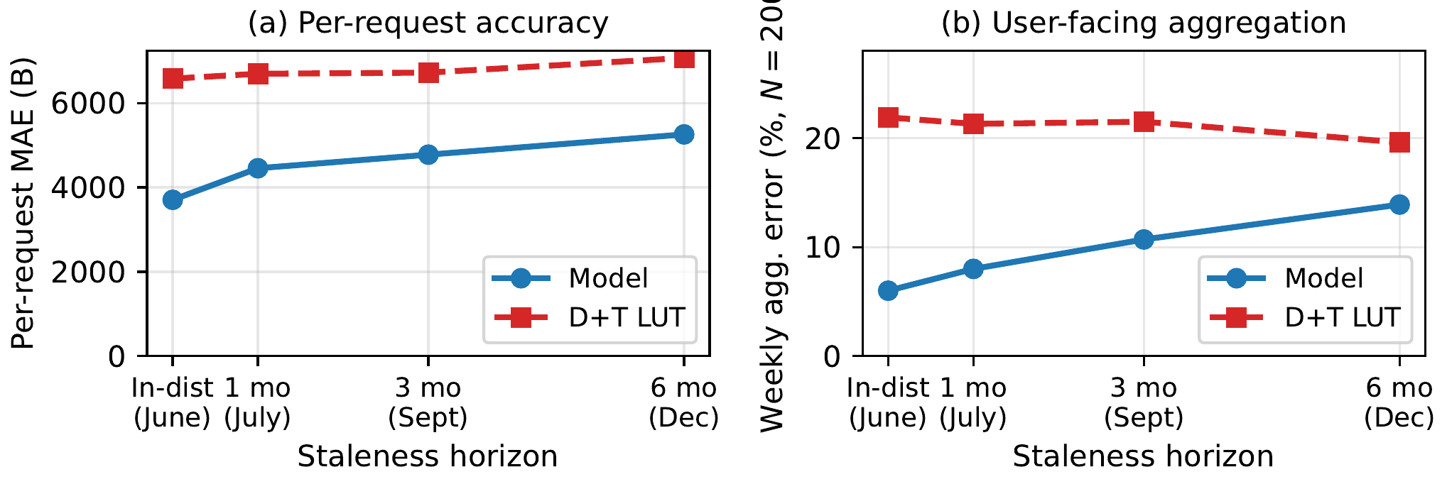
A random test split rewards a model on data that churns. The deployed estimator faces drift: tracker SDKs version their endpoints, and URL paths the model trained on go stale. To measure it, we evaluate the model on held-out HTTP Archive crawls 1, 3, and 6 months out — the worst-case staleness window a quarterly-retrained estimator would ever see. The per-request advantage over the domain+type LUT holds at +33.5% (1 month), +28.9% (3 months), +25.6% (6 months). On the user-facing weekly aggregation it erodes more gently — +13 pp, +10.8 pp, +5.7 pp — staying positive throughout. URL path churn, not domain churn, drives the decay, and the 3-month aggregation gap of +10.8 pp is what sets the quarterly retraining cadence.
Validating the deployment scenario directly
The whole project rests on one transfer assumption: labels learned from a Chrome-based HTTP Archive crawl apply to Firefox’s blocked requests. We don’t assert it — we test it two ways.
Per-URL byte agreement (does the same URL return the same bytes across browsers?). We fetched 46 representative tracker URLs paired across Firefox and Chrome and compared response sizes. The median byte ratio is 1.000, and 97.8% of URLs agree within 5%. The single outlier is Google reCAPTCHA at 0.63, documented rather than hidden. Tracker responses are server-determined and browser-invariant, exactly as the covariate-shift framing requires.
In-page Firefox crawl (does the model help on real Firefox traffic?). We crawled 35 traffic-publisher pages with headless Firefox via Playwright under Moto G4 mobile emulation (matching the training crawl’s conditions), and evaluated on the resulting 6,172 tracker requests across 499 domains — the actual deployment distribution, not held-out HTTP Archive rows. Per individual request the LUT is slightly better here (7,423 vs 8,367 bytes), because this harder distribution has more unseen paths. But on the weekly aggregation users actually see, the model preserves a 7–9 percentage-point advantage (N=200 uniform: 23.4% vs 31.3%; domain-correlated: 38.2% vs 47.5%). The model’s bias cancels under summation where the LUT’s compounds — the same mechanism, holding on real Firefox-served pages.
Deployment
The model integrates into the new-tab privacy widget. Integration is planned, not yet scheduled, but the architectural decisions are made.
Distribution. Model updates ship via Firefox Remote Settings, the same infrastructure used to distribute the Disconnect list. Quarterly retraining means a new model file is pushed alongside the next Disconnect list refresh. No browser update is required for a model change.
Inference path. When Enhanced Tracking Protection blocks a request, Firefox accumulates the cost prediction in the background. The block decision is unchanged — it remains a deterministic check against the Disconnect list. The model runs after the block, asynchronously, and updates the user’s weekly tally. The user never waits on inference. The aggregation layer that feeds the tally is the same metrics service I built for the count version of the widget.
Feature availability. Every input the model needs is already exposed by Firefox’s nsIChannel and nsILoadInfo interfaces at the point where ETP intercepts a request: the request URI maps to all URL features, the content policy type to resource type, the loading principal to initiator type, the HTTP method directly. No new instrumentation is required.
Model format and performance. XGBoost exports cleanly to ONNX as a ~500 KB artifact. Measured on commodity x86 over 10,000 calls (CPU-bound, single-thread, no GPU): median 50 µs, p99 93 µs per inference, resident memory ~5 MB loaded once at startup. Latency is far below any meaningful budget for a background task.
Size context. The path-level lookup table that achieves comparable accuracy would extrapolate to roughly 187 MB at full deployment scale — 350× the size of the model. The cost model adds a ~500 KB artifact next to the Disconnect blocklist to enable a feature the blocklist alone cannot provide. That ratio — same accuracy, 1/350th the size — is the case for ML over a table.
The negative finding: domain-level estimation does not need ML
We did not start with per-request prediction. The initial framing was domain-level scoring: assign each tracker domain a static cost based on aggregated HTTP Archive features, ship the result as a lookup table, no inference required. This is a simpler formulation, and it would have been the right one if it worked.
It did not work, but the way it failed is informative. Of 4,592 candidate tracker domains, only 48% had Lighthouse CPU timing measurements; the remaining 52% fell below Lighthouse’s ~50 ms reporting threshold and were structurally inexpensive in a way no machine learning model could discover from features. A Kolmogorov-Smirnov test confirmed the two populations were feature-distinct on all 19 candidate dimensions (). The unmeasured population’s feature vectors clustered at global-fallback values; the measured population’s vectors were genuinely informative.
We attempted self-training to bridge the gap: pseudo-label the unmeasured population using a model trained on the measured one, iterate. Three iterations of self-training produced zero improvement in MAE, because high-confidence pseudo-labels concentrated entirely among already-inexpensive domains where a simple rule worked as well as a learned model.
The diagnostic that emerged: ML adds value over a lookup table when there is a genuine prediction gap, when labels are absent for the deployment population and feature variance within key categories is too large for lookup to capture. The domain-level formulation failed this test. The per-request formulation passes it. Blocked requests have no response, so labels are structurally absent; within-domain URL variance is three orders of magnitude, far too large for any tractable lookup table. Reformulating the problem from domain-scoring to per-request prediction was the move that made machine learning the right tool.
Limitations
Deploy transfer size only. Timing metrics like TTFB and total load time depend on network conditions and device hardware that vary across the user base, while HTTP Archive collects from a fixed test environment (Moto G4, cable connection). Timing predictions are therefore standardized-condition estimates, not personalized predictions for a specific user. We recommend deploying transfer size and download duration only.
Cascading blocking effects. Our predictions cover only the directly-blocked request. In practice, blocking a tag manager or consent provider prevents an entire chain of downstream tracker requests from ever being issued. The aggregated weekly total is therefore a lower bound on true bandwidth saved by ETP, not the actual quantity. Measuring the cascading multiplier would require paired crawls and is orthogonal to per-request prediction.
Server-side variation. A/B tests, geo-targeting, and SDK versioning cause the same URL to return different payloads on different requests. This is irreducible from the model’s perspective: no pre-response feature can predict server-side randomization. Aggregation across many requests mitigates the impact in expectation.
No effect on blocking decisions. The model estimates the cost of an already-decided block. It does not influence what gets blocked. A miscalibrated estimate produces a misleading aggregate, never an over-block or under-block. The privacy guarantee of ETP is preserved by construction.
Calibration in the mid-range. The model is well-calibrated for near-zero beacons and for large script bundles, the two modes of the response distribution. For predicted sizes in the 500-byte to 5 KB range (small JSON responses, CSS files, redirect bodies) the model systematically underpredicts. Aggregation across requests partially cancels this bias, but per-request estimates in this range should be treated as order-of-magnitude rather than precise.
Adversarial robustness out of scope. The threat model is honest measurement. We do not model adversaries that craft URLs to game the cost estimator.
What I built
End-to-end on this project:
- The new-tab privacy widget itself (UI component, metrics service, top-trackers database, aggregation pipeline). The artifact that surfaces ETP to the user at all.
- The model: feature pipeline, training, evaluation, hyperparameter tuning, the loss-function ablation, the negative finding on domain-level estimation, the temporal and correlated-browsing robustness checks.
- The paper write-up (linked below).
Tim Huang (Senior Staff Engineer, Mozilla Privacy) co-designed the feature set with me and led the C++ side of the Gecko integration; I paired on the integration but did not write the runtime glue myself. The widget redesign work is documented separately on the Privacy Metrics Widget page.
Going deeper
The slide deck I presented to the Privacy team on 2026-04-29 covers the headline results. The four articles in the index below cover the project in depth.
The new-tab widget that consumes the model’s output is documented separately under Privacy Metrics Widget: the redesigned component, the metrics service that aggregates predictions, the top-trackers database, and the anti-tracking database flush logic.