Hand-Crafted Features and Tree Models
Methods
We train an XGBoost gradient boosted tree regressor to predict transfer_bytes from features observable before a response arrives. The target is zero-inflated (39.5% exact zeros, mostly beacons) and right-skewed (median 43 bytes, mean 13,607 bytes, max 14 MB). The feature set is 85 dimensions across five groups: domain target-encoding, TF-IDF/SVD embeddings of URL path tokens (50 dims), URL structure (path depth, length, query-parameter count, file extension), request metadata (resource/initiator type, HTTP method), and a small set of hand-curated URL-pattern regex flags.
Final configuration: 500 trees, max depth 8, learning rate 0.05, early stopping on a validation fold, Tweedie loss with variance power p=1.5. Tweedie loss requires strictly positive targets; we offset transfer_bytes by +1 during training and subtract 1 from predictions.
Baseline Comparison
We evaluate the model against a ladder of lookup-table baselines of increasing granularity on the held-out test split (Table 2). MAE is in bytes; the Size column is the full-population artifact size, which is the deployment constraint. Spearman rho measures ranking quality.
| Approach | Size | MAE | 95% CI | Spearman rho |
|---|---|---|---|---|
| Global median | <1 B | 19,905 | --- | --- |
| Domain LUT | 88 KB | 9,008 | --- | --- |
| Domain+type LUT (deployed baseline) | 114 KB | 6,802 | [6,633, 6,977] | 0.94 |
| Path LUT (fallback) — not deployable | 187 MB | 4,326 | [4,154, 4,516] | 0.93 |
| XGBoost Tweedie | 500 KB | 4,246 | [4,079, 4,442] | 0.93 |
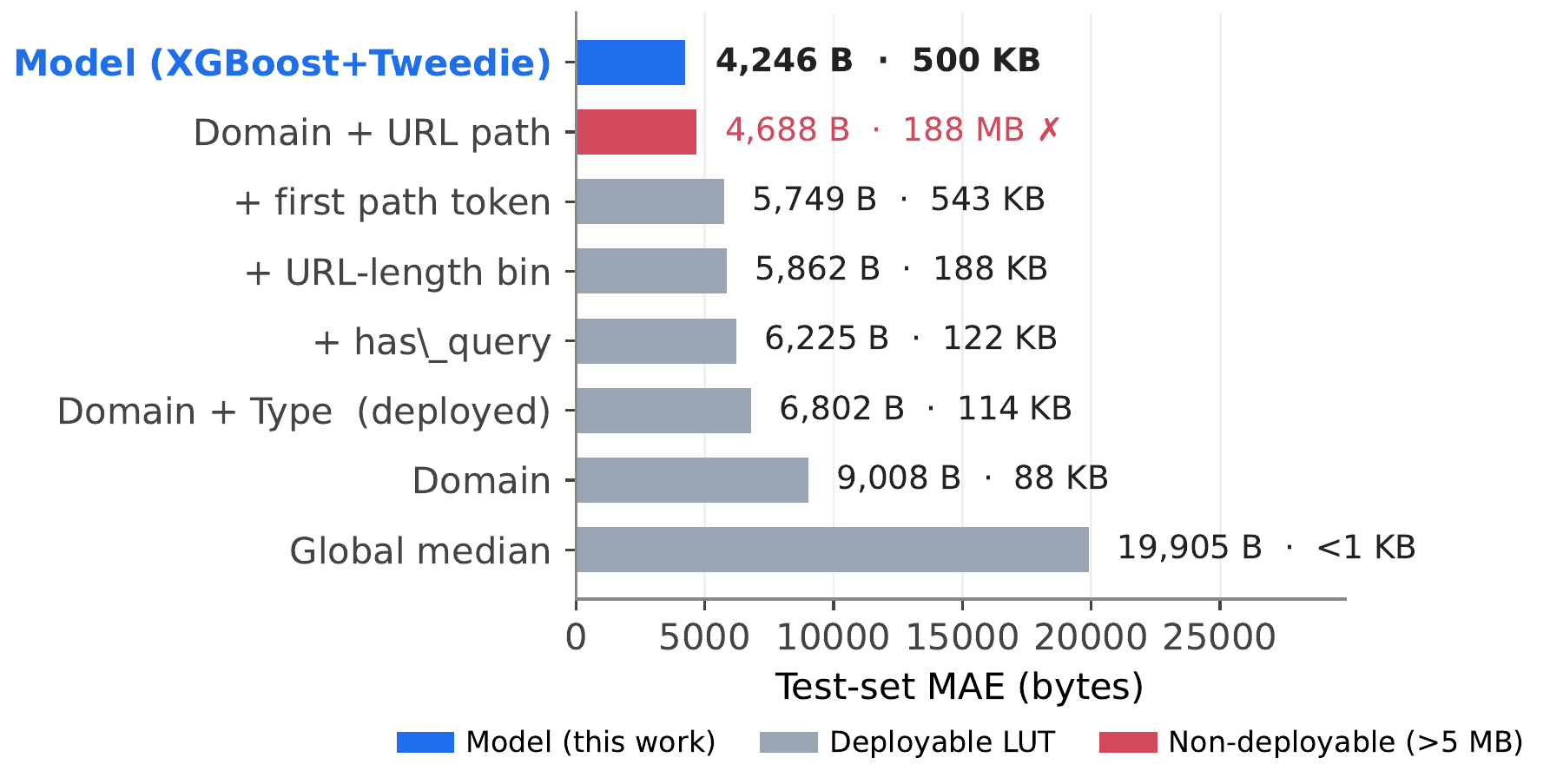
The XGBoost Tweedie model reaches MAE 4,246 bytes, a 37.6% reduction over the deployed domain+type lookup table (MAE 6,802) at a comparable 500 KB artifact size. The more important comparison is against the path-level lookup table: that table reaches 4,326 bytes — essentially the same accuracy as the model — but weighs 187 MB at full deployment scale, 350× larger than the model. The model lands within 2% of the path LUT’s accuracy while being the only entry in the ladder that achieves URL-level accuracy at a size that fits in Firefox’s Remote Settings envelope. The figure above plots the whole ladder on MAE × artifact-size axes: the model dot is the lone point in the low-MAE, low-size corner.
A linear baseline is not competitive on this data. A Brave-style Ridge regression on the same pre-response features reaches MAE 9,651 — worse than the lookup table it would replace (6,802), a 42% regression. Least-squares on a target with mean 13 KB and max 14 MB is dominated by the heavy right tail, and no linear combination of pre-response features tracks that tail closely enough to cancel the squared-error penalty. This is why the problem needs a loss matched to the target distribution, not a generic regressor.
Loss Function Ablation
The choice of loss function dominates all other design decisions.
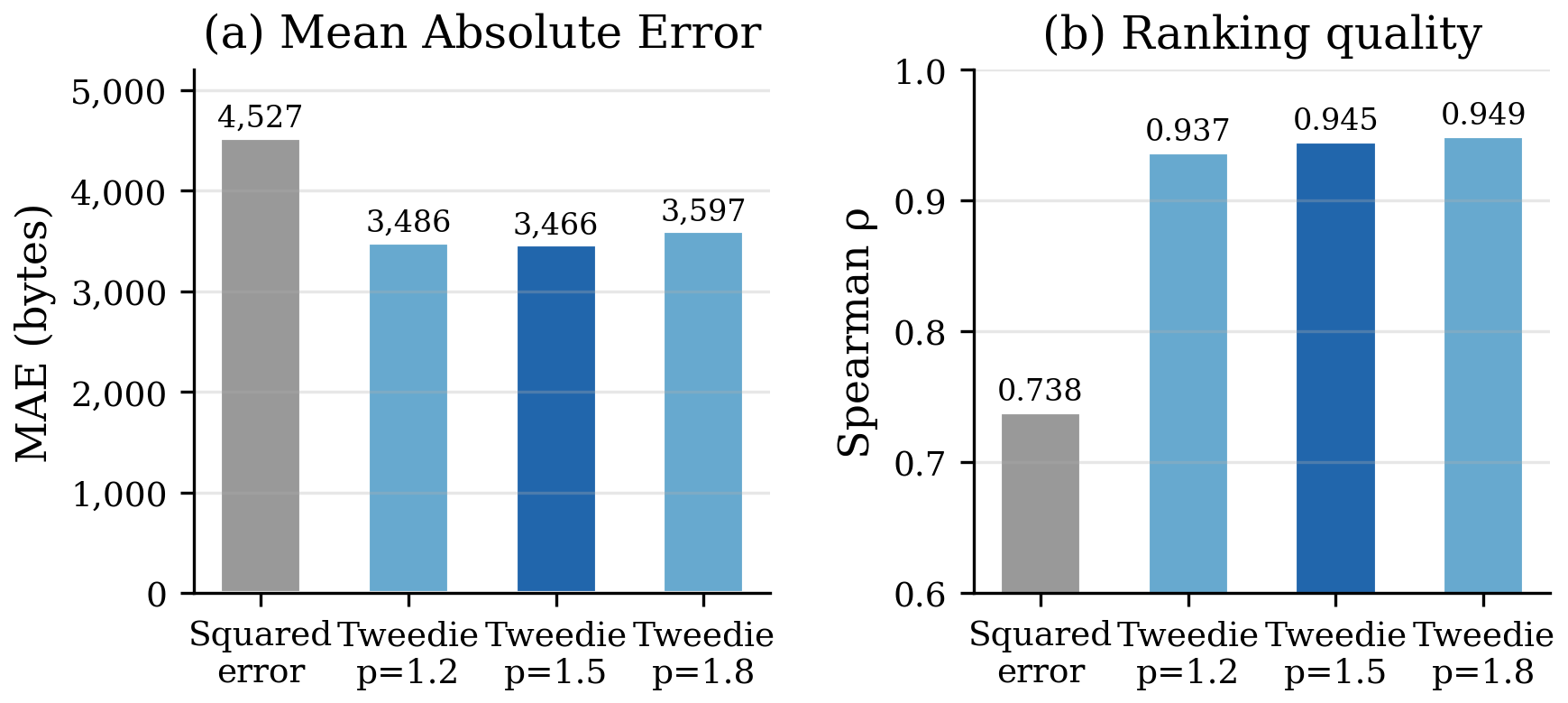
Two properties of the target distribution drive the loss choice. First, 39.5% of responses are exact zeros — beacons fired purely for their side effect on the server. Standard squared-error regression treats these as ordinary observations and pulls predictions toward them. Second, the non-zero tail is heavy: mean 13 KB, max 14 MB. Squared error trains a model that splits the difference between the spike at zero and the heavy tail and gets neither right.
Tweedie regression is the standard treatment for distributions with this exact shape — a point mass at zero plus a positive continuous tail — in actuarial science, where it has modeled insurance claims for decades. The variance power p ∈ (1, 2) controls how aggressively errors on large-magnitude predictions are weighted relative to errors on small ones; p=1.5 is the conventional middle ground. Holding architecture and features constant, an off-the-shelf squared-error baseline trails Tweedie at p=1.5 by roughly 23% — a gap that dwarfs the ~4% sensitivity to the Tweedie power within p ∈ [1.2, 1.8]. The loss is the dominant modeling choice; the power parameter is a rounding error by comparison.
Feature Ablation
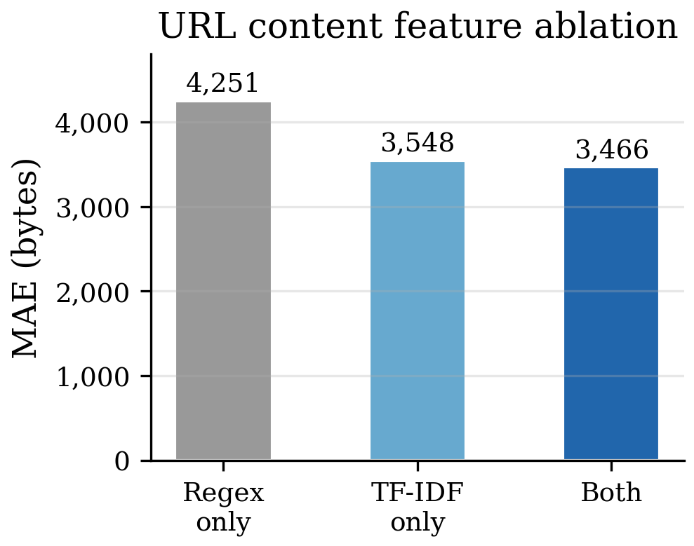
URL content features compose. Regex flags and TF-IDF embeddings each capture about half the URL-derived signal individually; the combined model reaches the headline MAE. TF-IDF subsumes most of the regex signal and adds patterns the researcher did not anticipate (for example, register-trigger paths associated with Privacy Sandbox). The learned URL representation does the work the hand-crafted flags can’t — which is the evidence that the model generalizes through URL structure rather than firing on a few hand-coded patterns.
Path Coverage Analysis
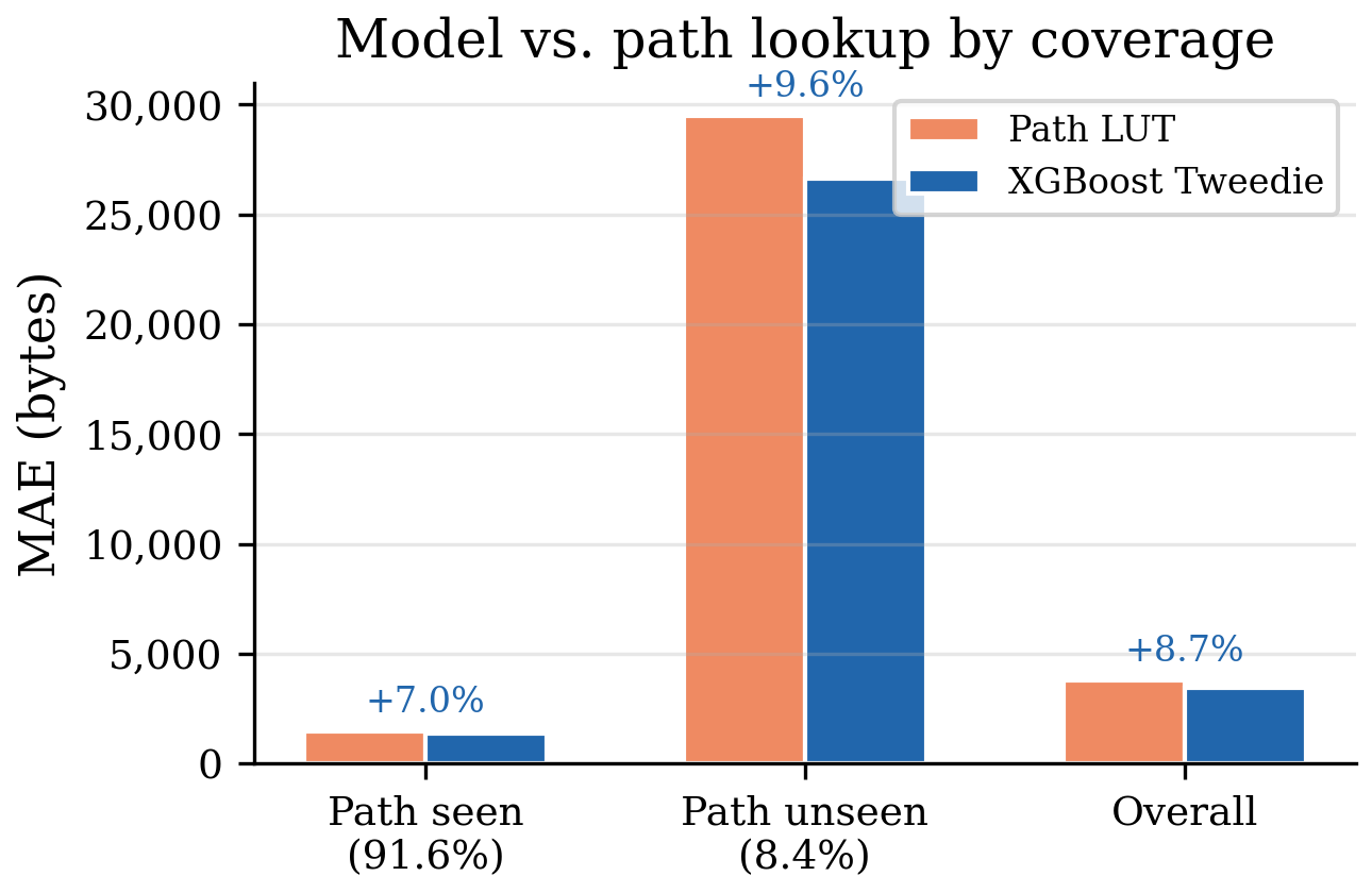
The cleanest test of whether the model generalizes — rather than memorizes — is to stratify the test set by whether the exact URL path was seen in training, and compare against the path-level lookup table, which on seen paths has the answer literally memorized (Table for path coverage).
| Subset | % of test | Path LUT MAE | Model MAE |
|---|---|---|---|
| Path seen | ~92% | 1,811 | 2,264 |
| Path unseen | ~8% | 33,471 | 27,224 |
On the ~92% of rows the path LUT can serve, the model matches path-level memorization — it is slightly behind per-request (2,264 vs 1,811 bytes), which is expected: the LUT has memorized the exact training median for those paths and the model is generalizing. But it matches that performance at a 350× smaller artifact, and with lower systematic bias (the model’s errors are closer to mean-zero, so they cancel under the weekly aggregation users actually see, where the LUT’s bias compounds). On the ~8% of rows with unseen paths — which are disproportionately expensive — the model clearly wins (27,224 vs 33,471), generalizing from URL structure and domain statistics where the table can only fall back to a coarse aggregate.
The honest read: the model does not beat a memorized lookup table on its home turf. It ties it there, at a fraction of the size, and pulls ahead exactly where memorization breaks down (unseen paths) and where the user actually reads the number (aggregation). Laplace add-k smoothing of the path LUT does not close the gap, confirming that learning URL structure beats regularizing exact-key memorization.
Resource Type Analysis
Per-type MAE, comparing the deployed domain+type LUT to the model (Table 3):
| Resource type | n (test) | LUT MAE | Model MAE | vs. LUT |
|---|---|---|---|---|
| Script | 144,676 | 12,996 | 3,135 | +75.9% |
| CSS | 6,142 | 6,222 | 2,084 | +66.5% |
| HTML | 92,438 | 2,246 | 1,294 | +42.4% |
| Image | 136,698 | 8,330 | 7,428 | +10.8% |
| Other (beacon) | 98,617 | 16 | 16 | +4.6% |
| Text | 42,984 | 292 | 303 | −3.8% |
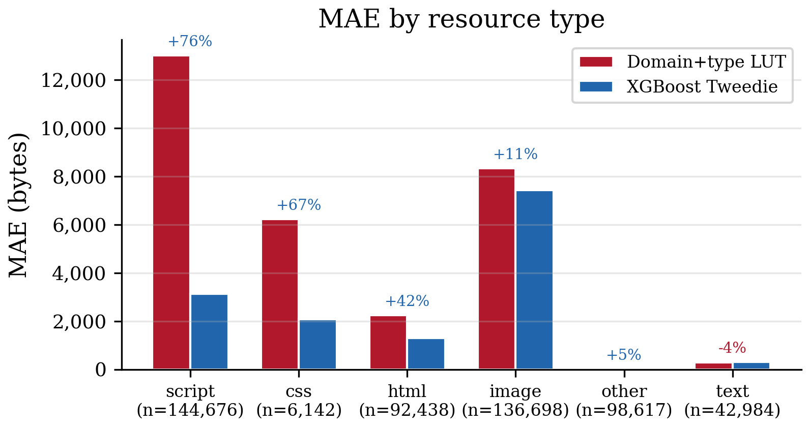
The model’s value concentrates on the high-cost, high-variance, URL-discriminative types: scripts (+75.9%) and CSS (+66.5%), which are exactly the high-byte classes from the per-category analysis. On beacons and short text responses there is no improvement — the LUT’s near-zero prediction is already near-optimal, and on text the model is fractionally worse (−3.8%). This is the correct failure mode: the model gives up nothing that matters, because the types it loses on contribute negligibly to the user-facing aggregate. Reporting the bucket it loses on is the point — the gains are credible because the losses are shown.
Aggregation Accuracy: the user-facing number
Users see a weekly aggregate (“Firefox saved you 2.3 MB”), not individual predictions. Per-request errors cancel under aggregation if they are approximately mean-zero. We simulate weekly browsing by sampling N blocked requests with replacement, summing predicted and true transfer sizes, and computing percentage error over many trials. We test both uniform sampling and domain-correlated sampling, since real users return to a small set of sites rather than drawing uniformly (Table 4).
| N | Model (uniform) | LUT (uniform) | Model (correlated) | LUT (correlated) |
|---|---|---|---|---|
| 50 | 6.8% | 20.8% | 14.2% | 34.5% |
| 100 | 6.3% | 20.9% | 12.5% | 34.2% |
| 200 | 6.0% | 21.9% | 12.9% | 36.4% |
| 500 | 5.1% | 23.2% | 11.2% | 36.7% |
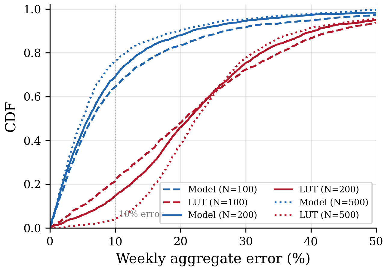
This is the most counterintuitive — and most important — result. Per-request, the model and the LUT are closer than the headline suggests. But under aggregation they diverge for a reason that is about bias, not noise. The LUT’s errors are systematic (it always predicts the conditional median, underpredicting scripts and overpredicting beacons), so they compound under summation; the model’s errors are approximately mean-zero, so they cancel. At N=200 the model lands within 6.0% of the true weekly total against the LUT’s 21.9%, and the gap widens with more requests because the LUT’s bias accumulates while the model’s noise washes out.
The advantage also widens under domain-correlated browsing — the realistic case — because the LUT’s per-domain bias compounds harder when requests concentrate on fewer domains, while the model retains within-domain discriminative signal from URL features. Low bias beats low variance once you sum.
Temporal Generalization
The headline is computed on a random split of the June 2024 crawl the model trained on. A deployed estimator faces a harder condition: the world drifts. To measure it, we evaluate the June 2024 model on held-out HTTP Archive crawls 1, 3, and 6 months later — the worst-case staleness window a quarterly-retrained estimator would ever see.
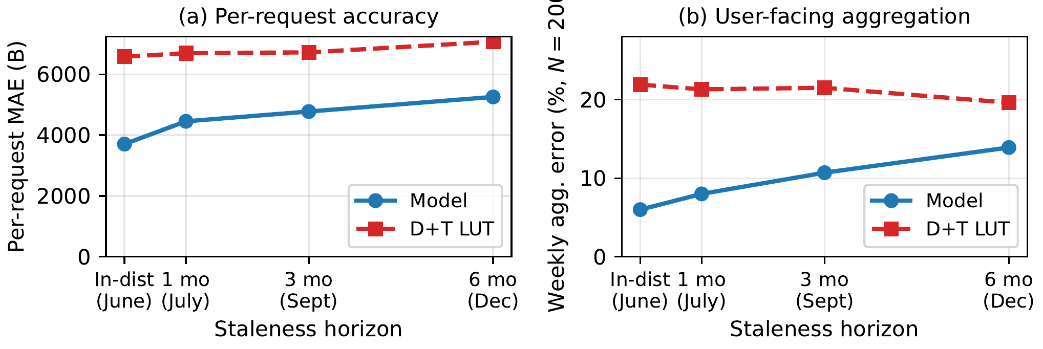
The model holds a per-request advantage of +33.5% at 1 month, +28.9% at 3 months, and +25.6% at 6 months over the domain+type LUT. In absolute terms, per-request MAE degrades from 4,454 (1 month) to 5,256 (6 months) — still beating the LUT by roughly a quarter at the far end. On the user-facing weekly aggregation the advantage erodes more gently: +13 pp at 1 month, +10.8 pp at 3 months, +5.7 pp at 6 months, staying positive throughout. URL path churn in versioned script bundles, not domain churn, drives the decay. The 3-month aggregation gap of +10.8 pp is what justifies a quarterly retraining cadence, bounding deployed-model staleness at three months.