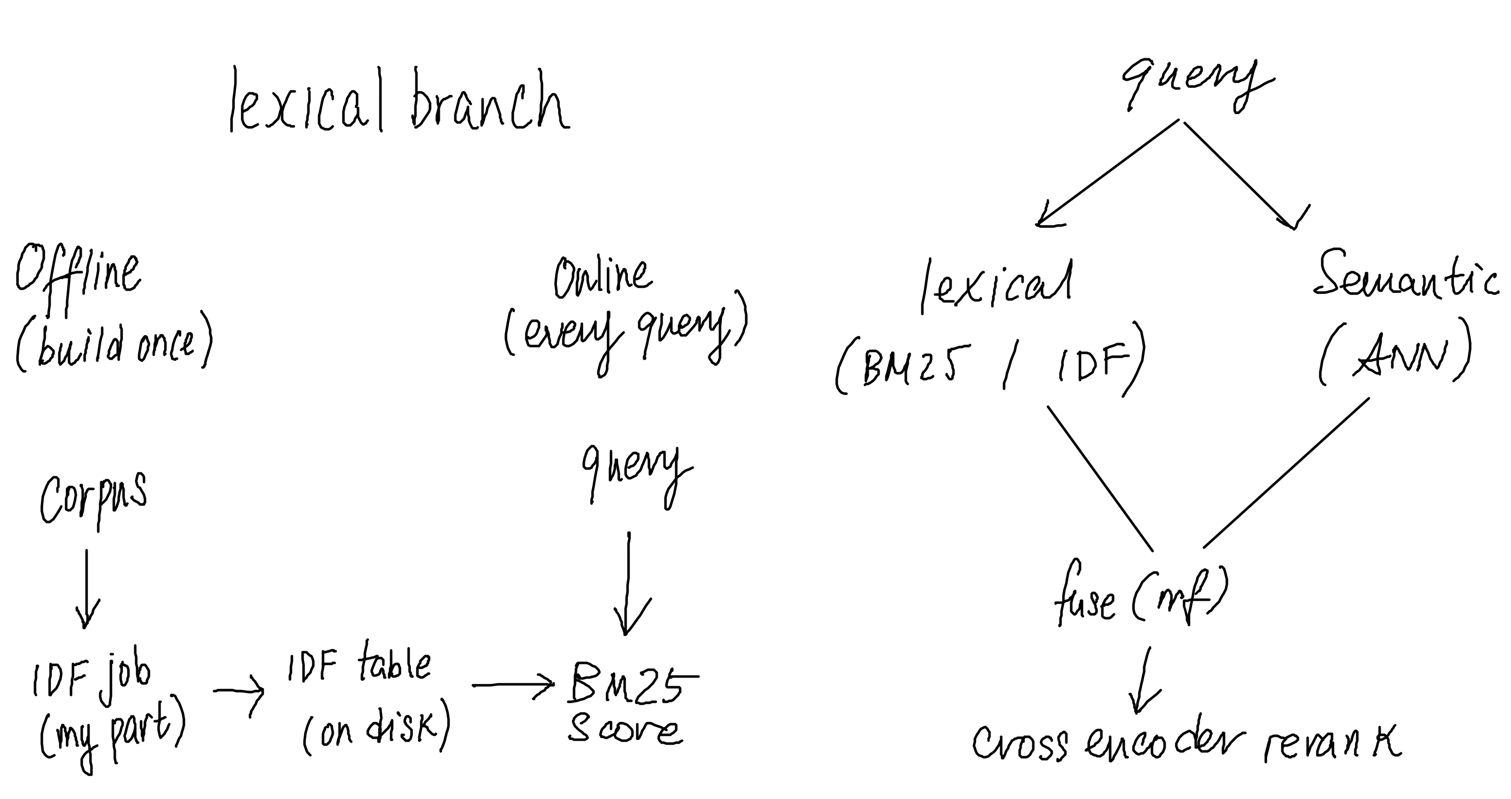
Lexical Retrieval: Index

Lexical retrieval is the arm that matches the actual words. It is the friars’ idea from the top-level map: a word maps to the places it appears, and you rank by the words a document shares with the query. This page is where I worked out what that arm looks like when it is built seriously, and the three places the naive version fell over on me, because each place I got stuck turned out to be where one of the leaves below came from.

The naive version is honest and it gets most of the way. For each document, count how many query words it contains, and rank by the count. Someone searches refund policy and back come the documents containing refund and policy, most matches first. It is roughly grep | sort | uniq -c, and on a small corpus with a literal query it actually works. Then I pushed on it.

Where it broke first: scanning every document is too slow

The naive loop walks every document for every query. A hundred documents, fine. Ten million and the user has closed the tab before the loop finishes. What fixes it is turning the problem inside out, which is exactly the move the friars made by hand: instead of storing, per document, the words it contains, store, per word, the documents that contain it. That is the inverted index, and it is the one data structure that makes lexical search fast. A query word becomes an instant lookup of the documents that could possibly match, and the documents that share no words with the query are never touched at all.

Everything else in this territory assumes the inverted index already exists, so it is where the depth starts. See the inverted index.

Where it broke next: not all matched words are worth the same

The naive count treats every shared word as equal, so a document matching the scores the same as a document matching refund. That is plainly wrong once you look at it. the is in nearly every document and tells you nothing about which one is relevant; refund is in few and tells you almost everything. The arm has to weight rare matched words far above common ones.

The surprising thing is that this exact intuition was made precise more than fifty years ago. Karen Spärck Jones, in a 1972 paper on what she called term specificity, argued that a term’s weight should be an inverse function of how many documents it appears in. That is inverse document frequency, IDF, the rarity signal that knows the is worthless and refund is gold. Pair it with term frequency (how often the word appears in this document) and you get TF-IDF, generally credited to Gerard Salton’s work on the SMART system. See TF-IDF.

TF-IDF gets two things wrong in practice, and fixing them is BM25, the function that has been the lexical default for about two decades. TF-IDF lets term frequency grow without limit, so a document that says refund ten times scores ten times higher, when really the first occurrence told you almost everything and the tenth told you nothing new. And it has no sense of document length, so a long document racks up matches just by being long. BM25 fixes both with two tunable knobs, saturation and length normalization. The name is the part I did not expect: it came out of the Okapi retrieval system at City University London in the early 1990s, built by Stephen Robertson and Steve Walker, and “BM25” is short for Best Match 25, the 25th weighting formula they tried. The default ranking function of the field is a numbered experiment that stuck. See BM25.

Underneath the formula there was a subtlety I had to stop and check. IDF has several variants and they are not interchangeable. The classic textbook form can go negative for very common terms, which a production engine usually does not want, so real systems use a non-negative variant with a smoothing term. And when one part of a system computes IDF and another part consumes it, the two formulas have to agree exactly. Confirming they match is a real task, not an assumption. See IDF variants.

Where it broke worst: “the words” is a lie

This is the break the textbooks skip and the one the day job is built around. Everything above quietly assumes I know what the words in a document are. I do not. Splitting on whitespace is not tokenization. A real analyzer is a pipeline: lowercase, fold accents, strip possessives, drop stop words, and reduce words to their stems so that running, runs, and ran collapse to one token. Refund, Refunds, refunding, and REFUND have to become the same thing, or they are four different words to the index and the rarity statistics for each one are wrong.

The part that turned this from a definition into something I lost sleep over is the agreement requirement. The tokenizer that builds the IDF table, the tokenizer that indexes the documents, and the tokenizer that processes the incoming query all have to produce identical tokens. If they disagree by a single rule, the query word and the indexed word fail to match, or the IDF weight gets looked up under the wrong key, and every score comes out quietly off with no error anywhere to tell you. When the canonical analyzer lives in one runtime (often the JVM, Lucene lineage) and the statistics pipeline lives in another (often Python), reproducing identical tokens across the two is the hardest single decision in this whole territory, which is why it is the deepest leaf. See tokenization and analysis.

A thing I did not expect: IDF buys speed too

I had been thinking of IDF purely as a quality signal. It is also what lets a retriever skip work. An algorithm like WAND uses the IDF weights to compute, for each document it has not fully scored yet, an upper bound on the score that document could possibly reach. If that bound is below the worst score already in the running top-k, the document cannot make the cut, so the retriever skips it without ever fully scoring it. Accurate IDF improves the ranking and the latency at the same time, which gave me a concrete operational reason to care about getting the weights right, not just an abstract one. See WAND and skip-based retrieval.

How the pieces sit together

Raw text and the incoming query both pass through the same analyzer, which has to produce identical tokens on both sides or the whole arm scores against the wrong vocabulary. The analyzer’s tokens feed two things built offline: the inverted index, which records which documents contain each token, and the corpus statistics, which record how rare each token is as IDF. At query time the retriever looks up the postings and the IDF weights, scores with BM25, and returns a ranked list, while WAND uses the IDF-derived score bounds to skip documents that cannot reach the top-k.

OFFLINE  (build, ahead of any query)

  docs ──▶ analyze ──┬──▶ inverted index   (token ──▶ which docs)
                     └──▶ IDF statistics   (token ──▶ how rare)


ONLINE  (one query)

  query ──▶ analyze ──▶ look up postings ──▶ BM25 score ──▶ ranked list
            ▲             + IDF weights        ▲
            │                                  │
  same analyzer as offline,          WAND uses IDF bounds to skip
  identical tokens or it breaks      docs that can't reach top-k

What kept surprising me is which half of this is hard. The math of what to compute, TF-IDF and BM25 and the choice of IDF variant, has been solved for years. The hard part in production is everything around the math: making the tokens agree across runtimes, computing the corpus statistics as a batch job that fits in memory, and shipping the resulting table to the serving layer without corrupting it. That last cluster is a data-engineering problem and it lives one level up in the indexing pipeline. The contract for the artifact connecting the two, the table mapping each term to its weight, is the IDF artifact.

This arm does not stand alone. It is half of hybrid search. Its blind spots, paraphrase and synonymy and meaning with no shared words, are what the semantic arm covers, and its strengths, rare exact terms and identifiers and precision on literal matches, are what semantic search misses. Up one level to the whole map.

Index

• The Inverted Index. The data structure that makes lexical search fast: store, per word, the documents that contain it. A worked three-document inversion, the postings list, and the design choices hiding inside a posting.
• TF-IDF. How lexical search learned to weight words: term frequency for how much a document is about a term, inverse document frequency for how much the term tells you anything at all, and the product that made the two work together. A worked toy corpus, the 1972 lineage, the one definition that quietly decides every weight, and what changed when I ran the whole thing over fifty-eight real documents.
• BM25. TF-IDF with the two things it gets wrong in practice fixed: term-frequency saturation, so the tenth occurrence of a word stops counting like the first, and length normalization, so a long document cannot win on bulk. The Okapi history, the k1 and b knobs and what each one does, and the saturation curve and short-document rescue watched on a real corpus.
• IDF Variants and the Agreement Contract. There is no single IDF formula. The textbook log(N/df), the classic BM25 form that can go negative, the non-negative Lucene form with its +1, and the smoothed sklearn form all disagree most exactly where stop words live. Why the variants exist, and a measured demonstration of which formula mismatch between builder and consumer is harmless and which silently reverses a query.
• Tokenization and Analysis. The break the textbooks skip: "the words in a document" is not a given, it is the output of an analyzer pipeline, and every IDF weight is only valid if the analyzer that builds the table, the one that indexes documents, and the one that processes queries all produce identical tokens. The pipeline stage by stage, a measured demonstration that a one-rule disagreement misroutes a quarter of query tokens, and the cross-runtime parity problem that hides behind "wire in the analyzer."
• WAND and Skip-Based Retrieval. Why accurate IDF buys speed and not just relevance. WAND uses per-term score upper bounds, derived from IDF, to prove a document cannot reach the top-k without fully scoring it, and skips it. The bound, the pivot, a measured skip rate on a real corpus, and the reason the savings come from IDF skew: a query mixing a rare term with common ones prunes the most.