Lexical Retrieval
Lexical retrieval matches the words the query actually contains, as opposed to matching its meaning. It is the older half of search, and it is the half that most write-ups introduce, dismiss in favour of embeddings, and then quietly reintroduce when they discover embeddings cannot find an error code.
The naive version: for each document, count how many query terms it contains, rank by the count. On a small corpus with a literal query this works. Four things break it, and each break produces a component of the real system.
1. The inverted index
The naive loop touches every document for every query, which is the cost the whole structure exists to avoid. The fix is to invert the mapping: instead of storing, per document, the terms it contains, store, per term, the documents that contain it.
That is the inverted index. Each term maps to a postings list, the set of documents containing it, usually with the position and frequency of each occurrence.
"refund"  ──▶  [ doc 3 (×2), doc 17 (×1), doc 402 (×5), ... ]
"chargeback" ─▶ [ doc 17 (×1), doc 88 (×3) ]
"the"     ──▶  [ doc 1, doc 2, doc 3, ... every document ]
A query becomes a lookup of a few postings lists and a merge, and documents sharing no terms with the query are never touched. Cost scales with the number of documents containing the query terms rather than with the corpus.
The structure carries its own hint about what comes next. The postings list for the contains everything, so it costs the most to process and tells you the least. That observation is the whole of the next section.
2. Inverse document frequency
Counting matched terms equally means a document matching the scores like a document matching chargeback, which is the failure the weighting exists to correct.
A term’s value as a signal is inverse to how many documents contain it. A term in every document separates nothing. A term in three documents out of fifty thousand almost fully determines the answer. Weighting a match by the rarity of the matched term is inverse document frequency, and the standard form is
idf(t) = log(N / df(t))where N is the corpus size and df(t) is the number of documents containing t. The logarithm is there because the raw ratio is too aggressive: without it, a term appearing in one document out of a million would outweigh a term appearing in a hundred by a factor of a hundred, and the difference between very rare and extremely rare does not carry that much information.
Multiplying term frequency by inverse document frequency gives TF-IDF, which is the correct idea and is not what anyone should ship. It has two specific failures, and the fix for both is the function that actually runs in production.
3. BM25
BM25 is TF-IDF with two specific repairs and two knobs that control them. It came out of the Okapi system at City University London in the early 1990s, from Stephen Robertson, Steve Walker and colleagues, building on probabilistic relevance work with Karen Spärck Jones going back to the 1970s. “BM” is Best Match and 25 is a version number: the twenty-fifth weighting scheme they tried. The default ranking function of lexical search for the last three decades is a numbered experiment that landed, and knowing that deflates the formula usefully. It is not derived from first principles. It is two repairs to TF-IDF, packaged with two interpretable knobs.
Repair 1. Term frequency has to saturate. Raw term frequency grows without limit, so a document using a query term a hundred times scores a hundred times a document using it once. That claims a page mentioning gradient a hundred times is a hundred times more about gradients, which is false. The first occurrence establishes the topic, the fifth confirms it, the fiftieth adds nothing.
The repair runs term frequency through a saturating function:
tf_factor = tf * (k1 + 1) / (tf + k1)Both numerator and denominator grow with tf, so the ratio approaches a ceiling of k1 + 1 rather than running away. The constant k1 sets how fast: roughly the term frequency at which the curve reaches half its climb. Typical values sit near 1.2. Sending k1 to infinity removes the saturation and recovers raw term frequency, which is the tell that this is a knob on TF-IDF rather than a different function.
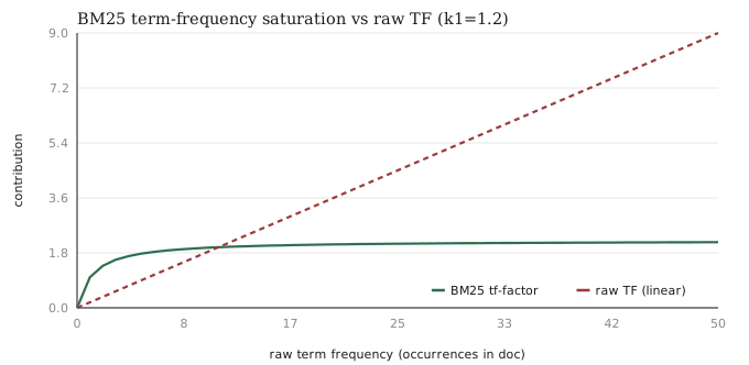
| raw tf | 1 | 2 | 3 | 5 | 10 | 20 | 50 | 100 | ∞ |
|---|---|---|---|---|---|---|---|---|---|
| tf-factor | 1.000 | 1.375 | 1.571 | 1.774 | 1.964 | 2.075 | 2.148 | 2.174 | 2.200 |
| gain over previous | – | +0.375 | +0.196 | +0.203 | +0.190 | +0.111 | +0.073 | +0.026 | → 0 |
Measured at k1 = 1.2. The second occurrence adds 0.375. The hundredth adds 0.026, less than a tenth of what the second was worth. Raw TF-IDF would have scored the hundred-occurrence term roughly fifty times higher than the two-occurrence one.
Repair 2. Long documents win by being long. A long document accumulates higher term frequencies because it has more words, so it scores higher without being more relevant. The repair normalizes against document length, folded into the same denominator:
                              tf * (k1 + 1)
score(t, d) = idf(t) * --------------------------------------
                        tf + k1 * (1 - b + b * (dl / avgdl))
dl is this document’s length, avgdl the corpus average, and the ratio is how this document compares to typical. b runs from 0 to 1 and controls how much length matters: at b = 0 length is ignored entirely, at b = 1 it applies in full. The usual setting is 0.75, partway on, because full normalization over-corrects and punishes genuinely thorough documents.
The mechanism is that a long document inflates its own denominator, so each term contributes less. It has to use the term proportionally more rather than absolutely more. The correction asks for density, not bulk.
avgdl is a corpus-wide statistic, so length normalization cannot be computed by a document about itself. Like inverse document frequency, it is build-time work, and it is the second quantity in the formula that forces a batch job to exist.
Set k1 to ten thousand and b to zero and BM25 reproduces raw TF-IDF ordering exactly. Both repairs off, and the function becomes the one it was repairing.
Both knobs are genuinely corpus-dependent and are tuned against a labelled relevance set rather than guessed. Low k1 suits corpora where one mention already signals relevance, such as titles or short documents. High b suits corpora with wide length variance. The defaults are defensible starting points and “the default holds up” is a claim to verify on your own data.
4. The idf variants, and the parity they require
The inverse document frequency formula has several forms in real use. The classic is log(N / df). Lucene and systems following it use a smoothed, non-negative variant:
idf(t) = log(1 + (N - df + 0.5) / (df + 0.5))The 0.5 terms prevent division by zero for unseen terms. The 1 + keeps the result non-negative, which matters because the unsmoothed probabilistic form goes negative for terms appearing in more than half the corpus, and a negative weight means matching a term actively lowers a document’s score, which is rarely intended.
The variants differ modestly in ranking quality and the choice is not where the difficulty is. The difficulty is that the same variant has to be used in both places.
Term statistics are computed by a build-time job. Scoring happens in the serving engine. If the job computes log(N/df) and the engine expects the smoothed form, every weight is wrong by an amount that varies per term, and the ranking degrades in a way that looks like generally mediocre relevance rather than like a bug. The system reports no error. This is the agreement problem in its simplest form, and the defence is an explicit contract: the artifact states which variant produced it, and the consumer asserts the variant it expects.
5. WAND, the skipping algorithm rarity weights permit
Rarity weighting has a second payoff, and it turns a quality mechanism into a performance one.
Because each term’s inverse document frequency bounds how much that term can contribute to any document’s score, a retriever can compute the maximum score a partially-scored document could still reach. If that ceiling falls below the current tenth-best score, the document cannot enter the top ten and can be skipped without being fully scored.
That is WAND, and its consequence is that the postings lists you most want to avoid processing, the ones for common terms, are exactly the ones whose low weights let the skipping fire. Good weights make retrieval both more relevant and faster, which is not the usual shape of that trade.
6. The bag-of-words ceiling
BM25 is the best the lexical side gets, and it is a bag-of-words function. It does not know that running and ran are the same word, that NYC and New York are the same place, or that a query and a document can mean the same thing while sharing no terms.
The first of those is the analyzer’s job, and BM25 silently assumes it already happened. The rest is what the semantic arm exists for.
A worked example
Scoring the same corpus with raw TF-IDF and with BM25 at k1 = 1.2, b = 0.75, then looking for queries where the ranking changes.
The corpus is 58 documents averaging roughly 690 tokens, with the shortest near empty and the longest over 3,000. That spread is what makes length normalization observable.
On the query embedding:
| rank | TF-IDF, no length normalization | BM25 at b=0.75 |
|---|---|---|
| 1 | 1,715 tokens | 1,715 tokens |
| 2 | 2,510 tokens | 2,510 tokens |
| 3 | 2,724 tokens | 385 tokens, up from rank 7 |
Raw TF-IDF’s top three are all long documents, the kind that mention embeddings often because they mention everything often. BM25 keeps the two genuinely on-topic long pages and pulls a 385-token page from seventh into third. A short focused document that uses the term densely beats long documents that use it merely often, which is b doing exactly its job.
The same pattern held on other queries: BM25 consistently promoted shorter, denser documents over longer ones that had accumulated frequency through bulk.
Then the degeneracy check. Setting k1 = 10000 and b = 0, disabling both repairs, reproduced raw TF-IDF’s ordering on all ten top positions. Both patches off, and BM25 becomes the function it was patching.
The scorer itself is small enough to state completely:
import math

def idf(t, N, df):                                     # Lucene's smoothed non-negative form
    return math.log(1 + (N - df + 0.5) / (df + 0.5))

def bm25(tf, dl, idf_t, avgdl, k1=1.2, b=0.75):
    # tf    : term frequency in this document
    # dl    : this document's length in tokens
    # avgdl : average document length across the corpus
    norm = 1 - b + b * dl / avgdl                      # >1 for long docs, shrinking their score
    return idf_t * (tf * (k1 + 1)) / (tf + k1 * norm)
These numbers come from a small pure-Python implementation over a 58-document corpus with a deliberately crude analyzer, so the exact values are corpus-specific. What generalizes is the direction and the degeneracy check.