Semantic Retrieval
Lexical retrieval cannot match text that means the same thing in different words. A user asks how do I get my money back and the document that answers is titled refund policy. No content word is shared, so term matching returns nothing and the user is told the answer does not exist when it is sitting in the corpus.
That gap is not an edge case. Users describe problems in their own words and documentation is written in the vocabulary of the people who built the product, so the mismatch is the normal condition rather than the exception.
Closing it requires matching on something other than the surface form.
1. What an embedding is
An embedding is a function from text to a fixed-length vector, a point in a space of a few hundred to a few thousand dimensions. What makes it an embedding rather than an arbitrary hash is one trained property: texts that mean similar things map to points that are close together, and texts that mean different things map to points that are far apart.
The description “the meaning of the text as numbers” is true enough to be useless. The specific version is better and explains the failures later on.
The geometry is learned contrastively. The model is shown many pairs known to be similar, a question and its correct answer, a sentence and its paraphrase, and many pairs known to be dissimilar, then adjusted so similar pairs come out close and dissimilar pairs come out far. Over enough pairs it generalizes and places unseen text near its paraphrases.
The model is never told what meaning is. It is shown which things should be close and learns coordinates that make them so. An embedding space is the residue of millions of “these two go together, these two do not” judgments, and that framing does real work: it predicts that the space is good exactly where the training pairs were dense and unreliable where they were sparse.
This is why an embedding matches how do I get my money back to refund policy. Somewhere in training the model saw refund-shaped questions paired with refund-shaped answers and learned to place that whole region of phrasings in one neighbourhood. The match is geometric because the training made the geometry encode the pairing.
2. Cosine similarity
If meaning is a location, similarity is a distance. The metric used almost everywhere is cosine similarity: the dot product of two vectors divided by the product of their lengths, which is the cosine of the angle between them. It runs from 1 for vectors pointing the same way, through 0 for perpendicular, to −1 for opposite.
Cosine measures direction and ignores magnitude, which is the right choice because the direction of an embedding is what training shaped to carry meaning, while the length tends to reflect incidental properties like text length. Two documents on the same topic, one a paragraph and one a page, should be near each other, and a metric sensitive to magnitude would separate them for the wrong reason.
In practice vectors are usually normalized to unit length at index time, after which cosine similarity and dot product are the same operation, and the dot product is cheaper.
3. Approximate nearest-neighbour search
Retrieval now means finding the vectors nearest the query vector. Done exactly, that is a comparison against every vector in the corpus, and scanning the whole corpus per query is what a search system exists to avoid. Ten million comparisons per query is affordable in a way that ten million cross-encoder passes is not, but it still does not fit a few-hundred-millisecond budget alongside everything else.
High-dimensional geometry offers no clean way out. The tree structures that make low-dimensional nearest-neighbour search efficient degrade toward linear scan as dimensions rise, because in high dimensions almost every point is roughly equidistant from every other. Exact nearest-neighbour search in a few hundred dimensions has no good algorithm.
So the field gave up exactness. Approximate nearest-neighbour search returns most of the true nearest neighbours most of the time, for a fraction of the work. The quality measure is recall: the fraction of the true top-k that the approximate search actually returned. Recall against cost is the only dial that matters here.
Two structures dominate.
- Inverted file indexes partition the vectors into cells by clustering, each with a centroid. A query compares against the centroids, picks the nearest few cells, and searches only inside those. The
nprobeparameter sets how many cells to search: more probes, more recall, more cost. Vectors near a cell boundary whose true neighbours sit in an unprobed cell are the misses. - Navigable small-world graphs, of which HNSW is the standard, build a graph where each vector links to some near neighbours, with long-range links in upper layers. A search enters at the top and greedily walks toward the query, descending layers. HNSW generally gives excellent recall at high speed and is the default in most vector databases, at the cost of more memory and slower builds than an inverted file index.
The choice between them is measured on the real corpus rather than argued: inverted file indexes are cheaper to build and combine well with compression, HNSW gives better recall per unit of search time.
Compression compounds with both. Product quantization splits each vector into subvectors and replaces each with a codebook entry, cutting memory by an order of magnitude at some recall cost. Reducing dimensions before indexing is nearly lossless for recall in many cases. Each compression step is another small recall sacrifice, which is why the honest framing of this whole layer is to fix a target recall and minimize cost, or fix a cost and maximize recall, and never to claim the approximation is free.
4. The literal-token failure
Embeddings go vague exactly where precision matters most, which is why serious systems do not run this arm alone. Ask for an error code, an API method, a product SKU, a version string, a function signature, a rare proper noun, and the result is something thematically adjacent and useless. ENOENT has no synonyms. A user who types it wants the document containing that exact string, and a model trained to place similar meanings nearby will happily return documents about file errors in general.
The mechanism follows directly from how the geometry was trained. Contrastive training builds a space where nearby means similar in meaning, and a rare literal token has no meaningful neighbourhood: it appeared too infrequently in training to have a well-shaped region, so it gets placed by weak generalization from its surface form and context. The failure is structural, not a quality problem with a particular model. A better embedding model has the same weakness at a different threshold.
There is a second and quieter failure. Embeddings compress a document to a fixed-length vector, and a long document containing several distinct topics gets a vector that is a blur of all of them, close to nothing in particular. Chunking documents into passages before embedding is the standard mitigation, and it is the reason retrieval usually operates on passages while results are presented as documents, which is where the collapsing stage in the funnel comes from.
Lexical retrieval fails on paraphrase. Semantic retrieval fails on literals. They fail on disjoint sets of queries, which is exactly the condition under which running both beats running either.
A worked example
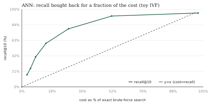
Measuring the recall-versus-cost curve directly, on 4,000 vectors clustered into 64 cells, searching for the top ten and varying how many cells get probed.
| nprobe | avg comparisons | cost vs exact | recall@10 |
|---|---|---|---|
| 1 | 127 | 3% | 16.4% |
| 2 | 189 | 5% | 24.9% |
| 4 | 315 | 8% | 40.6% |
| 8 | 565 | 14% | 59.0% |
| 16 | 1,063 | 27% | 78.6% |
| 32 | 2,062 | 52% | 95.9% |
| 64 | 4,064 | 102% | 100.0% |
Two things read straight off the table.
Probing every cell gives perfect recall and costs more than brute force, because you pay to compare against all 64 centroids and then against every vector anyway. The approximation is only worth anything when it is genuinely approximate.
The curve is steeply concave. Sixteen probes buy 78.6% of the true neighbours for 27% of the cost. Doubling to 32 probes buys another 17 points of recall for double the work. Useful operating points sit in the middle, and the right one depends on what a miss costs downstream.
One caveat on these specific numbers: the test vectors were near-uniform random, which have almost no cluster structure and are therefore the worst case for a partitioning index. Real embeddings cluster hard, which is what makes this approach work in practice, so recall at low probe counts is pessimistic here. What generalizes is the shape of the curve.