Data Collection and Ground Truth Construction
There’s no labeled dataset of “tracker domain to performance cost.” So I built one from 348 million HTTP requests and Lighthouse audits on BigQuery.
The Problem
No one has published a dataset that maps tracker domains to their performance impact on web pages. The Disconnect list categorizes domains by privacy function. The third-party-web project1 tracks script execution time by entity. But neither produces what I actually needed: per-domain performance cost scores covering CPU and network overhead independently.
I had to construct the ground truth labels from raw web crawl data.
-
Patrick Hulce’s third-party-web project maps ~2,700 entity names to their associated domains, categorized by function (ad, analytics, social, etc.). This mapping is consumed by Chrome Lighthouse and DevTools to attribute performance costs to named entities rather than raw domains. ↩
Data Sources
HTTP Archive2 crawls millions of web pages monthly and stores the results in BigQuery. Four data sources feed the pipeline:
| Source | What it provides | Scale |
|---|---|---|
httparchive.crawl.requests | Per-request timing, transfer size, resource type, waterfall position | 348M rows, 374GB (2024-06-01 mobile crawl) |
httparchive.crawl.pages | Per-page Lighthouse audit results as nested JSON | ~16M pages |
httparchive.almanac.third_parties | Entity-to-domain mapping from the third-party-web project | ~2,700 entities |
Disconnect services.json | Privacy categories for tracker domains | 4,387 domains |
I used the 2024-06-01 crawl (most recent with stable Lighthouse v12 data) and the mobile client, which is more representative of constrained devices and covers ~60% of HTTP Archive’s crawl.
-
HTTP Archive is a community-run project (started by Steve Souders) that crawls millions of URLs monthly using WebPageTest on Chrome, storing HAR files and Lighthouse audits in Google BigQuery. The annual Web Almanac is the canonical publication built on this data. ↩
Lighthouse Audit Schema
The first surprise came before I wrote any aggregation logic. My design doc, based on older HTTP Archive documentation and examples, assumed three Lighthouse audit names:
| Design doc assumed | Actual audit name (2024 crawl) |
|---|---|
third-party-summary | third-parties-insight |
render-blocking-resources | render-blocking-insight |
bootup-time | bootup-time (unchanged) |
Lighthouse renamed two of three audits at some point between the documentation I was referencing and the 2024 crawl. The only way to discover this was to explore the JSON structure interactively on BigQuery, extracting keys from the lighthouse column and checking what actually existed.
This is the kind of thing that burns hours if you don’t verify early. I was writing queries against audit names that no longer existed in the data.
Entity-Level Attribution
The second surprise was worse. The third-parties-insight audit doesn’t use domain names. It uses entity names from the third-party-web project:
{
  "entity": "Google Tag Manager",
  "mainThreadTime": 305.4,
  "transferSize": 98234,
  "blockingTime": 142.1
}
The key is "Google Tag Manager", not "www.googletagmanager.com". To map these back to domain-level scores, I needed the entity-to-domain mapping from httparchive.almanac.third_parties. This meant the third-party-summary audit couldn’t directly join to the request data on domain name; it needed an intermediate join through entity names.
For the bootup-time audit, the data uses URLs directly ($.url), so domain extraction is straightforward with NET.HOST(). This asymmetry between audits added complexity but was manageable once I understood the schema.
The Extraction Pipeline
Stage 1: Per-Request Feature Extraction
The first query pulls raw request-level signals for every HTTP request to a known tracker domain:
SELECT
  NET.HOST(req.url) AS tracker_domain,
  req.page,
  req.type AS resource_type,
  CAST(JSON_VALUE(req.payload, '$._bytesIn') AS INT64) AS transfer_bytes,
  CAST(JSON_VALUE(req.payload, '$._load_ms') AS INT64) AS load_ms,
  req.index AS waterfall_index,
  JSON_VALUE(req.payload, '$._priority') AS chrome_priority,
  JSON_VALUE(req.payload, '$._initiator_type') AS initiator_type,
FROM `httparchive.crawl.requests` req
WHERE req.date = '2024-06-01'
  AND req.client = 'mobile'
  AND req.is_root_page = TRUE
  AND NET.HOST(req.url) IN (
    SELECT domain FROM `httparchive.almanac.third_parties`
    WHERE category IN ('ad', 'analytics', 'social',
                        'tag-manager', 'consent-provider')
  )
This scanned 374GB and returned 348 million rows, covering every request to a third-party tracker domain across the entire mobile crawl. Cost: ~$1.87 on BigQuery.
Stage 2: Lighthouse CPU Extraction
The second query pulls per-script CPU breakdown from the bootup-time audit:
SELECT
  NET.HOST(JSON_VALUE(item, '$.url')) AS tracker_domain,
  COUNT(DISTINCT page) AS pages_with_data,
  AVG(CAST(JSON_VALUE(item, '$.scripting') AS FLOAT64))
    AS mean_scripting_ms,
  AVG(CAST(JSON_VALUE(item, '$.scriptParseCompile') AS FLOAT64))
    AS mean_parse_compile_ms,
  AVG(CAST(JSON_VALUE(item, '$.total') AS FLOAT64))
    AS mean_total_cpu_ms,
FROM `httparchive.crawl.pages`,
  UNNEST(JSON_QUERY_ARRAY(lighthouse,
    '$.audits.bootup-time.details.items')) AS item
WHERE date = '2024-06-01'
  AND client = 'mobile'
  AND is_root_page = TRUE
GROUP BY tracker_domain
Lighthouse only reports scripts that exceed a CPU threshold in the bootup-time audit. Domains that don’t appear here didn’t cross the reporting threshold, meaning “absent” is closer to “negligible CPU” than “unmeasured.” This distinction becomes critical later.
Stage 3: Domain-Level Aggregation
The aggregation collapsed 348 million request rows into 4,592 tracker domains (filtered to pages_seen_on >= 10 for statistical stability). This step runs in Python rather than SQL because it requires the Disconnect list fuzzy matching and percentile rank computation.
Disconnect List Fuzzy Matching
The initial naive join between HTTP Archive domains and the Disconnect list was disappointing:
Exact domain match: 92 matches out of 4,59292 matches. The problem: the Disconnect list uses base domains (doubleclick.net), but HTTP Archive records full subdomains (stats.g.doubleclick.net, td.doubleclick.net, pagead2.googlesyndication.com).
The fix was suffix matching: try progressively shorter domain suffixes until a match is found.
def match_disconnect_domain(tracker_domain, disconnect_domains):
    parts = tracker_domain.split(".")
    for i in range(len(parts) - 1):
        candidate = ".".join(parts[i:])
        if candidate in disconnect_domains:
            return candidate
    return None
stats.g.doubleclick.net tries stats.g.doubleclick.net (miss), then g.doubleclick.net (miss), then doubleclick.net (hit). After this fix: 3,686 matches (80% of domains). The remaining 906 domains are in HTTP Archive’s third-party categories but not on the Disconnect list.
Coverage Analysis
Not every domain has every type of data. This split defines the ML problem:
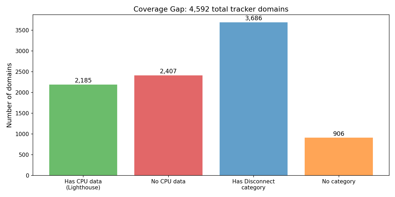
| Segment | Count | Meaning |
|---|---|---|
| Domains with Lighthouse CPU data | 2,185 (48%) | Real training labels for main_thread_cost |
| Domains without CPU data | 2,407 (52%) | Model predicts their scores |
| Matched to Disconnect list | 3,686 (80%) | Have privacy category features |
| Not on Disconnect list | 906 (20%) | In HTTP Archive’s tracker categories but not Disconnect |
Every domain has network data (transfer size comes from the request table), so network_cost has real labels for all 4,592 domains. But main_thread_cost only has ground truth for the 2,185 where Lighthouse reported CPU time. The model’s job is to predict CPU cost for the other 2,407 using only request-level features.
Missing Data and Label Noise
This was the most consequential data decision in the project.
The mistake: In my first training run, I filled missing CPU data with 0.0 and trained on all 4,592 domains. The 2,407 domains without CPU data got main_thread_cost = 0.0. The model reported Spearman rho = 0.825. Looked great.
The problem: 0.0 means “Lighthouse didn’t report CPU time,” not “zero CPU cost.” The model was learning fake labels.3 Those 2,407 domains were being treated as ground truth when they were assumptions. The model trained on “small transfer size correlates with zero CPU” because that’s what the fake labels said. But small transfer doesn’t mean zero CPU. bat.bing.com serves 258-byte stubs that trigger 105ms of scripting.
The evidence: When I evaluated only on the 328 test domains with real CPU data, rho dropped from 0.825 to 0.734. The inflated metric was coming from the model “correctly” predicting low scores for domains that had fake 0.0 labels.
The fix: Train main_thread_cost only on the 2,185 domains with real Lighthouse CPU data. Use the model to predict scores for the 2,407 without data.
| Metric | Before (fake 0s) | After (real data only) |
|---|---|---|
| Training set | 4,592 domains | 2,185 domains |
| Spearman rho (honest eval) | 0.734 | 0.767 |
| RMSE | 0.173 | 0.091 |
| MAE on real-data domains | 0.173 | 0.062 |
RMSE nearly halved. MAE improved 3x. And the rho on real data went up, not down, despite training on half the data. The fake labels were actively hurting the model.
-
For a thorough treatment of how label noise degrades model performance, see Frenay and Verleysen, “Classification in the Presence of Label Noise: A Survey” (IEEE TNNLS, 2014). Systematic label noise (like replacing missing values with a constant) is particularly damaging because it teaches the model a spurious pattern rather than adding random variance. ↩
Percentile Rank Construction
Percentile ranks convert raw milliseconds and bytes into [0.0, 1.0] scores that are robust to outliers and interpretable (“worse than X% of trackers”).
But here the fake-0 problem showed up again in the target construction. When I computed percentile ranks across all 4,592 domains, the 2,407 with “zero” CPU all tied at rank 0.0. The remaining 2,185 real domains got compressed into the [0.52, 1.0] range. The model was training on targets bunched in the upper half of [0, 1], wasting half the output space.
The fix: compute ranks only within the 2,185 domains with real CPU data.
has_cpu = df["mean_scripting_ms"].notna()

df.loc[has_cpu, "prank_scripting"] = (
    df.loc[has_cpu, "mean_scripting_ms"]
    .rank(pct=True, method="min")
)
This gives the training set a full [0, 1] range. Domains without CPU data get NaN for main_thread_cost; they’re the prediction targets, not the training labels.
For network_cost, all 4,592 domains have real network data, so ranks are computed over the full set with no issues.
Target Distributions
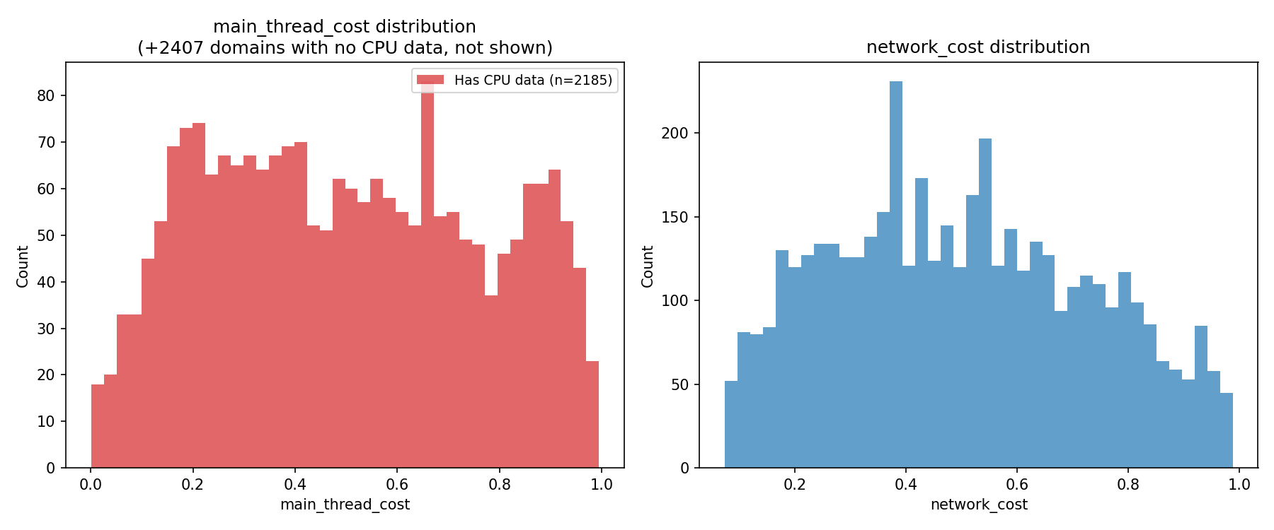
main_thread_cost (left): The 2,185 domains with Lighthouse CPU data are spread roughly uniformly across [0, 1]. This is what percentile ranking gives you: a flat distribution by construction. The 2,407 without CPU data are not shown; they have no score yet.
network_cost (right): All 4,592 domains have real network data. Distribution is roughly uniform with a slight right skew. Every tracker transfers something, so there’s no spike at zero.
The two distributions have very different shapes in raw space (before percentile ranking). CPU time is extremely right-skewed with a long tail of heavy SDKs. Network cost is more evenly distributed. Percentile ranking normalizes both to [0, 1], which is what the model trains on.
Score Validation
Before training any model, I checked the score profiles against domains where I had strong priors:
| Domain | main_thread_cost | network_cost | Expected |
|---|---|---|---|
googletagmanager.com | 0.92 | 0.90 | Heavy on both axes |
connect.facebook.net | 0.64 | 0.83 | FB SDK: heavy scripts, large transfer |
google-analytics.com | 0.53 | 0.46 | Moderate CPU (higher than I expected) |
bat.bing.com | 0.52 | 0.42 | Moderate CPU despite 258-byte transfer |
cdn.cookielaw.org | 0.79 | 0.84 | Consent: heavy script, big transfer |
The key validation is that the two dimensions produce different profiles for qualitatively different trackers. GTM is heavy on both. Analytics is moderate-moderate. Bing’s pixel is moderate CPU but low network. The profiles match reality, which means the labeling pipeline is working.