| 2026.03.28

Model Architecture and Training

The biggest script a domain serves is the single best proxy for CPU cost when you don’t have Lighthouse data. Everything else is noise.

Why XGBoost

The task is tabular regression: 19 numeric features in, one float out per target. The dataset is small (~2K-4.5K domains depending on the target). The models need interpretability for the downstream consumer (Firefox engineers deciding whether to trust the scores). I compared four options.

Option	Pros	Cons	Verdict
Ridge regression	Simple, fast, tiny model	Can’t capture feature interactions	Baseline only
Random forest	Handles nonlinearity; robust	Large model size; no native missing value handling	Inferior to XGBoost here
Small neural net	Could learn feature embeddings	Overkill for 19 features and ~2K samples; poor interpretability; larger model	Wrong tool
XGBoost	Best on small tabular data; native missing values; interpretable via SHAP; small ONNX export	No transfer learning	Selected

The critical factor was feature interactions.¹ A linear model can learn “high transfer size = high cost,” but it can’t learn “high script ratio + large size = high cost, but high script ratio + small size = low cost.” That interaction is real: a domain that serves many small scripts (like a retargeting pixel chain) behaves very differently from one that serves a few large scripts (like an ad SDK). XGBoost captures this with tree splits, and it does so efficiently on small datasets where neural nets would overfit.

Ridge regression turned out to be a strong baseline (rho=0.713 for CPU cost), which I’ll return to in the evaluation article. But XGBoost beat it by a meaningful margin on the target that matters most.

Chen and Guestrin, “XGBoost: A Scalable Tree Boosting System” (KDD, 2016). For systematic evidence that tree-based models outperform deep learning on medium-sized tabular data, see Grinsztajn, Oyallon, and Varoquaux, “Why do tree-based models still outperform deep learning on typical tabular data?” (NeurIPS, 2022), which benchmarks across 45 datasets and finds trees dominant below ~10K samples. ↩

Two Independent Models

I train two independent XGBRegressor models, one per target axis. Not a single multi-output model,² for several reasons:

Per-target tuning matters. main_thread_cost trains on 2,185 domains (only those with real Lighthouse CPU data). network_cost trains on all 4,592 (every domain has real network data). Different dataset sizes, different distributions, different optimal hyperparameters.
Independent failure modes. If one model turns out to be unreliable, I can drop it without retraining the other. In practice, network_cost turned out to be trivially solved while main_thread_cost required real effort.
Per-target SHAP analysis is cleaner when each model is self-contained. The features that drive CPU cost are completely different from the features that drive network cost.

Spyromitros-Xioufis, Tsoumakas, Groves, and Vlahavas, “Multi-target regression via input space expansion” (Machine Learning, 2016) systematically compare independent single-target models against methods that exploit inter-target correlations. They find independent models are competitive when targets have low correlation, which is exactly the case here, since CPU and network cost are largely independent. ↩

Training Data Selection

This was the single most impactful decision in the entire pipeline.

The dataset has 4,592 tracker domains. Of those, only 2,185 have real Lighthouse CPU data (they appear in the bootup-time or third-party-summary audits). The remaining 2,407 have main_thread_cost = 0.0, not because they truly cost zero CPU, but because Lighthouse didn’t measure them. They load after Lighthouse’s observation window, or they don’t trigger audits, or they only serve images.

Version 1 of the model trained on all 4,592 domains, including those fake zeros. It achieved a headline Spearman rho of 0.825 on the full test set. Looked great. But 340 of the test domains had those fake 0.0 labels, and the model “correctly” predicted low for them, inflating the metric.

Version 2 trained main_thread_cost only on the 2,185 domains with real Lighthouse data. The honest metric, evaluated only on domains where the label is real, improved from 0.734 to 0.751. The headline number went down, but the actual model got better. I cover this in detail in the evaluation article.

network_cost has no such problem. Every domain has real network data (transfer size, request count, bytes per page), so it trains on all 4,592 domains.

Hyperparameter Search with Optuna

Each target gets its own Optuna³ study with 5-fold cross-validation, optimizing for Spearman rank correlation. Not RMSE, not R-squared. Spearman rho, because the downstream use case cares about ranking (which trackers are most expensive on each axis), not about predicting exact scores.

import optuna
from scipy.stats import spearmanr
from sklearn.model_selection import KFold

def objective(trial):
    params = {
        'n_estimators': trial.suggest_int('n_estimators', 30, 200),
        'max_depth': trial.suggest_int('max_depth', 3, 7),
        'learning_rate': trial.suggest_float(
            'learning_rate', 0.01, 0.3, log=True
        ),
        'min_child_weight': trial.suggest_int('min_child_weight', 1, 20),
        'subsample': trial.suggest_float('subsample', 0.6, 1.0),
        'colsample_bytree': trial.suggest_float(
            'colsample_bytree', 0.5, 1.0
        ),
        'gamma': trial.suggest_float('gamma', 0, 5),
        'reg_alpha': trial.suggest_float('reg_alpha', 1e-8, 10, log=True),
        'reg_lambda': trial.suggest_float('reg_lambda', 1e-8, 10, log=True),
    }

    kf = KFold(n_splits=5, shuffle=True, random_state=42)
    scores = []
    for train_idx, val_idx in kf.split(X_train):
        model = xgb.XGBRegressor(
            **params,
            objective='reg:squarederror',
            tree_method='hist',
            random_state=42,
        )
        model.fit(
            X_train.iloc[train_idx], y_train.iloc[train_idx],
            eval_set=[(X_train.iloc[val_idx], y_train.iloc[val_idx])],
            verbose=False,
        )
        preds = model.predict(X_train.iloc[val_idx])
        rho, _ = spearmanr(y_train.iloc[val_idx], preds)
        scores.append(rho)

    return np.mean(scores)

study = optuna.create_study(direction='maximize')
study.optimize(objective, n_trials=100)

The search space is deliberately wide on regularization parameters (reg_alpha, reg_lambda, gamma) because small datasets can overfit quickly. Optuna’s tree-structured Parzen estimator navigates this efficiently. The training loss uses reg:squarederror for stable gradient descent, but the tuning objective is Spearman rho, the metric I actually care about.

Akiba, Sano, Yanase, Ohta, and Koyama, “Optuna: A Next-generation Hyperparameter Optimization Framework” (KDD, 2019). Optuna’s Tree-structured Parzen Estimator (TPE) navigates high-dimensional hyperparameter spaces more efficiently than grid or random search by modeling the conditional probability of good vs. bad configurations. ↩

Results

Target	Training Domains	Spearman rho	RMSE	MAE
main_thread_cost	2,185 (real CPU data only)	0.751	0.182	0.140
network_cost	4,592 (all domains)	0.999	0.010	0.007

The asymmetry is striking. Network cost is essentially a solved problem; the model reconstructs the target almost perfectly from transfer size features. CPU cost is the real modeling challenge, because the features available at inference time (request metadata, no Lighthouse) are indirect proxies for the thing you’re trying to predict (JavaScript execution time).

An rho of 0.751 means the model gets the CPU cost ranking right about 75% of the time. I think that’s good enough for the downstream use case: correctly identifying which blocked trackers were expensive and which were cheap. It won’t perfectly distinguish the 65th percentile domain from the 70th, but it will correctly separate a heavy tag manager from a lightweight pixel. I should note that 2,185 training samples with 19 features is on the thin side, and I’m relying on Optuna’s cross-validation to catch overfitting rather than doing a proper learning curve analysis. Something to revisit.

SHAP Analysis

SHAP⁴ (SHapley Additive exPlanations) decomposes each prediction into per-feature contributions. The summary plots reveal what each model actually learned.

main_thread_cost

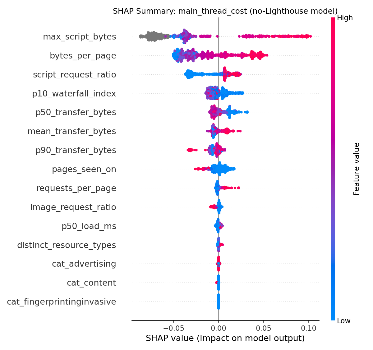
The top features by mean absolute SHAP value:

Rank	Feature	Mean \|SHAP\|
1	`max_script_bytes`	0.056
2	`bytes_per_page`	0.030
3	`script_request_ratio`	0.019

Everything else is at or near zero. The Disconnect categories (Advertising, Analytics, Social, etc.) barely register. The model learned one dominant pattern: the size of the biggest script a domain serves is the best available proxy for its CPU cost, when you don’t have Lighthouse timing data.

This makes intuitive sense. A large JavaScript file needs to be parsed, compiled, and executed. A domain serving a 170KB script is almost certainly running more expensive logic than one serving 2KB. bytes_per_page adds a cumulative signal (total load from this domain), and script_request_ratio adds a type signal (is this domain mostly scripts or mostly images?).

What surprised me is how little the Disconnect categories contribute. “Advertising” vs “Analytics” doesn’t predict CPU cost once you control for script size. The privacy taxonomy and the performance taxonomy are nearly orthogonal.

network_cost

The network cost SHAP is even more concentrated:

Rank	Feature	Mean \|SHAP\|
1	`p50_transfer_bytes`	0.096
2	`bytes_per_page`	0.084
3	everything else	~0.000

Two features explain essentially all of the model’s predictions. p50_transfer_bytes (median transfer size per request) and bytes_per_page (total bytes from this domain per page) together are network cost. This is why the model achieves rho=0.999: the target variable network_cost is a weighted percentile rank of these same transfer size signals. The model is recovering a near-deterministic relationship.

Lundberg and Lee, “A Unified Approach to Interpreting Model Predictions” (NeurIPS, 2017). SHAP connects game-theoretic Shapley values to local model explanations, providing consistent and theoretically grounded feature attributions. The TreeSHAP variant runs in polynomial time on tree ensembles. ↩

Feature-Target Relationships

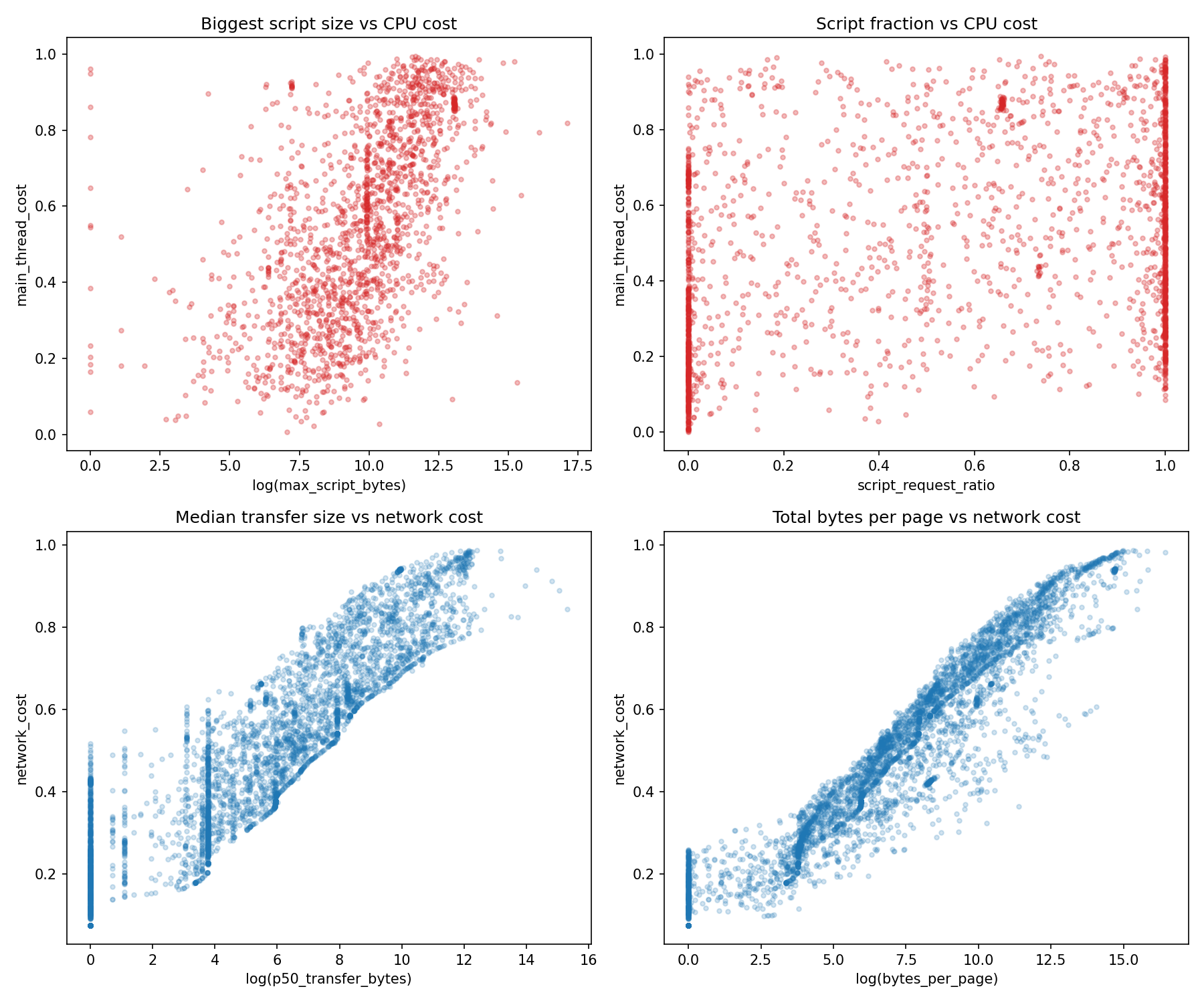
The scatter plots show why the two models have such different accuracy. The network cost features (transfer size, bytes per page) have a clear monotonic relationship with the target; you can almost draw a line through them. The CPU cost features (max script bytes, script ratio) have a much noisier relationship. Large scripts tend to be CPU-expensive, but some large scripts are mostly data (JSON payloads, configuration objects) while some small scripts trigger expensive event listeners, cookie operations, and beacon chains.

Prediction Accuracy

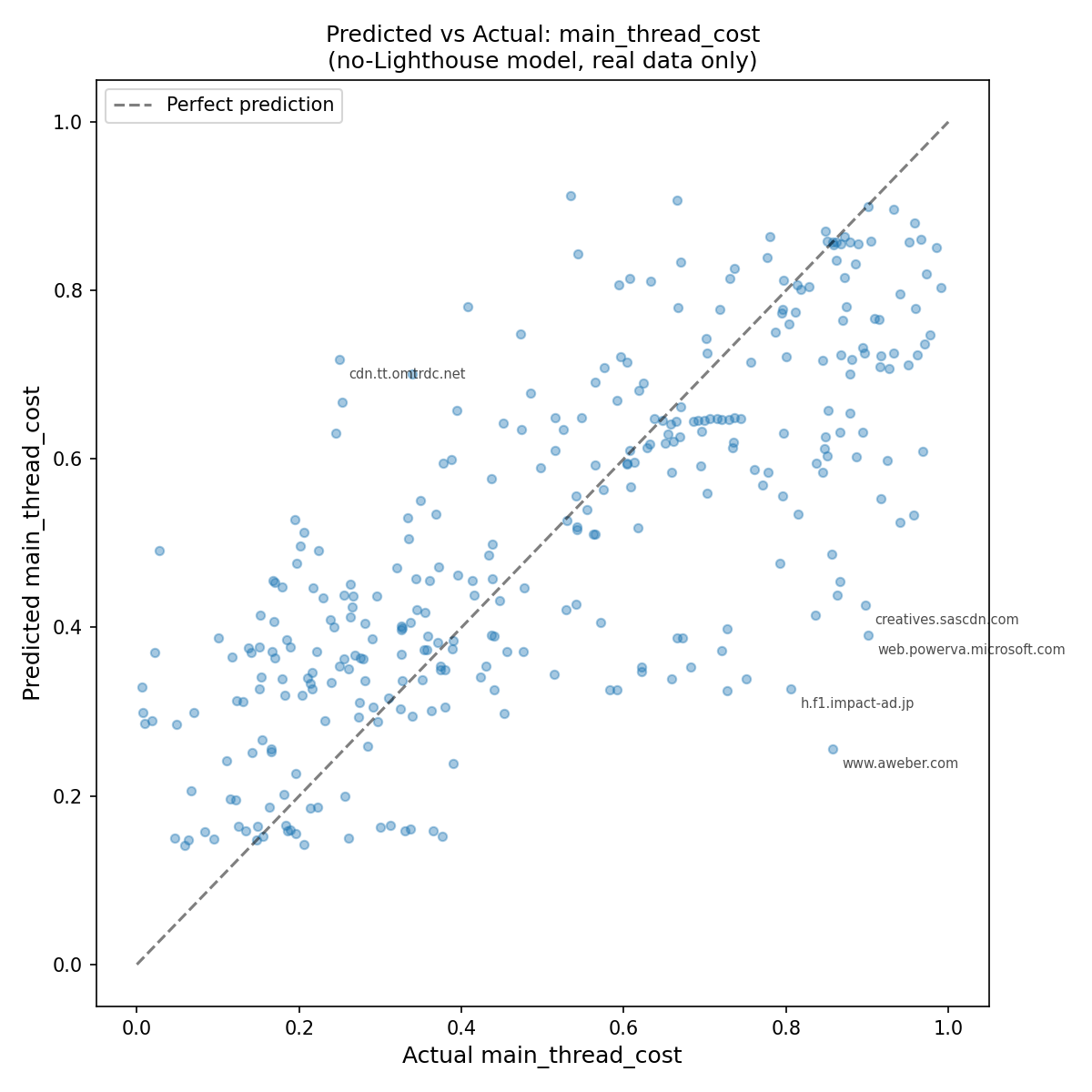
Predicted vs actual for main_thread_cost model

The 45-degree line is the ideal. Points above are over-predictions; points below are under-predictions. The model tracks well through the middle of the distribution but struggles at the extremes. Domains with very high actual CPU cost (above 0.8) are systematically under-predicted. The model doesn’t have strong enough signal from request metadata to identify the most expensive trackers. I examine these failure cases in the evaluation article.