Uncertainty Quantification
The point estimates were decent. But a single number per domain hides something important: how much does the model trust its own prediction?
I applied three techniques on top of the base XGBoost models, each building on the previous one. Quantile regression produces prediction intervals. Self-training tries to exploit the unlabeled data. Conformal prediction audits everything. The most interesting results were the ones I didn’t expect.
Quantile Regression
Instead of predicting one score per domain, predict three: the 10th percentile, median, and 90th percentile. If the interval is narrow, the model is confident. If it’s wide, the model is saying “I’m not sure about this one.”
XGBoost supports this natively.1 Set objective='reg:quantileerror' and pass the quantile level via quantile_alpha. No architecture changes, no custom loss functions. I trained 6 models total: 2 targets x 3 quantiles.
def train_quantile_model(X_train, y_train, quantile, base_params):
    model = xgb.XGBRegressor(
        **base_params,
        objective="reg:quantileerror",
        quantile_alpha=quantile,
        tree_method="hist",
        random_state=42,
    )
    model.fit(X_train, y_train)
    return model

for target in ["main_thread_cost", "network_cost"]:
    for q in [0.1, 0.5, 0.9]:
        model = train_quantile_model(X_train, y_train, q, params)
The p10-p90 interval should contain the true value about 80% of the time. That’s the target coverage.
Results
| Target | Coverage (p10-p90) | Mean width | Median rho |
|---|---|---|---|
| main_thread_cost | 0.680 | 0.413 | 0.745 |
| network_cost | 0.804 | 0.115 | 0.999 |
Two very different stories. Network cost intervals are tight (mean width 0.115) and well-calibrated (coverage 0.804, right on the 0.80 target). The model knows network cost and knows that it knows. Main thread cost intervals are wider (0.413) and under-covering (0.680 vs 0.80 target). The model is slightly overconfident about CPU predictions; it thinks its intervals are wide enough, but they’re not.
That 0.68 coverage is interesting. It means 32% of true CPU scores fall outside the predicted p10-p90 range. The noise in CPU prediction (redirect chains, cross-domain script attribution, dynamic loading) creates surprises that the model can’t flag in advance.
Per-domain interval analysis
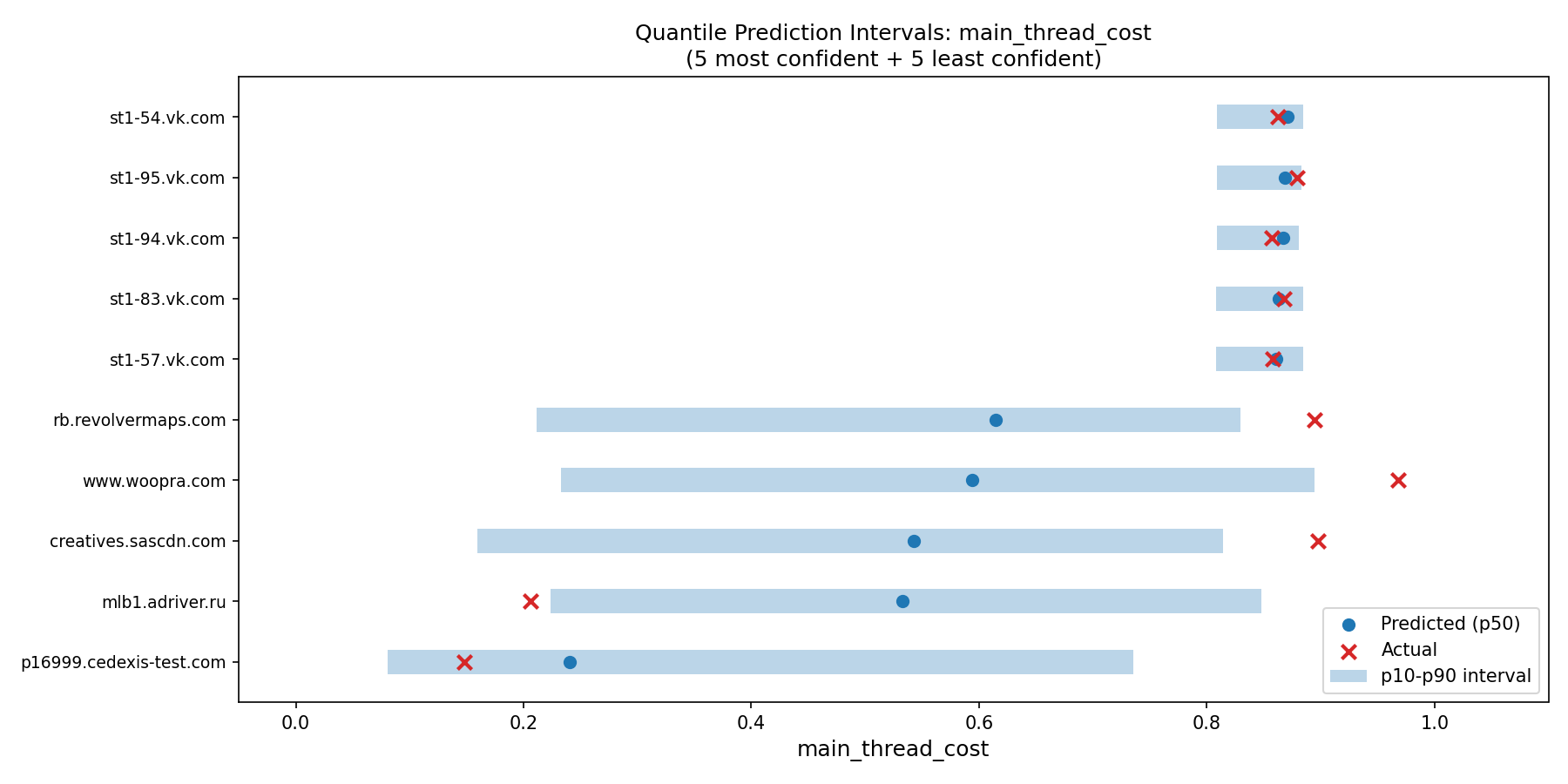
The most confident predictions (narrowest intervals) were VK social media domains. Consistent heavy scripts, predictable behavior. The model sees large max_script_bytes, high script_request_ratio, and knows exactly what to predict. Narrow blue bars, actual values landing right inside.
The least confident predictions (widest intervals) were Instagram CDN domains. The same CDN serves lightweight thumbnails on one page and heavyweight video players on another. The model can’t tell which pattern applies, so it hedges. Intervals spanning 0.3-0.4 of the full score range.
Interval width as uncertainty proxy
Does the model actually know when it’s uncertain? The width-error correlation for main_thread_cost is rho=0.280, positive but modest. Wider intervals do tend to correspond to larger prediction errors, but it’s not a strong signal. The model has some self-awareness of its uncertainty, not total self-awareness.
For network cost, the question barely applies. Errors are so small (max 0.039 across all test domains) that there’s nothing meaningful to correlate with interval width.
-
Quantile regression was introduced by Koenker and Bassett, “Regression Quantiles” (Econometrica, 1978). The asymmetric pinball loss function penalizes over- and under-predictions differently depending on the target quantile. XGBoost added native support via the
reg:quantileerrorobjective in version 2.0 (2023); see the XGBoost quantile regression tutorial. ↩
Semi-Supervised Self-Training
The setup looked textbook.2 1,857 labeled domains (with Lighthouse CPU data) and 2,407 unlabeled domains. Classic semi-supervised opportunity. The idea: train on labeled data, predict on unlabeled data, use the quantile intervals from above to select confident predictions (interval width < 0.30), add those as pseudo-labels, repeat for 5 rounds.
def self_train(df, params, n_rounds=5, max_width=0.30):
    for round_num in range(n_rounds):
        model = train_model(X_train, y_train, params)

        # Use quantile intervals for confidence
        q_models = train_quantile_pair(X_train, y_train, params)
        pred_lo = q_models["lo"].predict(X_unlabeled)
        pred_hi = q_models["hi"].predict(X_unlabeled)
        widths = pred_hi - pred_lo

        # Only add predictions the model is confident about
        confident_mask = widths < max_width
        X_train = pd.concat([X_train, X_unlabeled[confident_mask]])
        y_train = np.concatenate([y_train, pred_mid[confident_mask]])
        X_unlabeled = X_unlabeled[~confident_mask]
Results
| Round | Training size | Spearman rho | Added | Remaining unlabeled |
|---|---|---|---|---|
| Baseline | 1,857 | 0.751 | — | 2,407 |
| 1 | 1,867 | 0.751 | 10 | 2,397 |
| 2 | 1,884 | 0.747 | 17 | 2,380 |
| 3 | 1,902 | 0.745 | 18 | 2,362 |
| 4 | 1,949 | 0.749 | 47 | 2,315 |
| 5 | 2,228 | 0.751 | 279 | 2,036 |
Total pseudo-labels added: 371. Improvement in Spearman rho: exactly +0.000. Self-training had no effect.
Not a small effect. Not a marginal improvement. Zero. The metric didn’t move at all across five rounds and 371 additional training examples.
Analysis of null result
Self-training helps when unlabeled data comes from a different region of feature space than the labeled data, when the model would encounter new patterns it hasn’t seen. That’s not what happened here.
The unlabeled domains are unlabeled because they’re simple. Lighthouse didn’t report CPU time for them because they didn’t cross the reporting threshold. They’re tracking pixels, tiny beacons, cookie-sync endpoints, the boring tail of the distribution. The labeled set of 2,185 domains already covers the full spectrum, from near-zero to 7,000ms of CPU time. It contains pixels and heavyweight SDKs and everything in between.
Adding pseudo-labeled versions of “more boring domains” doesn’t teach the model anything new. The model already knows what boring looks like. It needs help with the hard cases, domains where request features don’t clearly indicate CPU cost, and those are exactly the domains where self-training can’t help, because the model’s predictions on them aren’t confident enough to use as labels.
This is a clean negative result. It’s more informative than not trying, because it confirms the labeled set is representative. The 1,857 domains with real Lighthouse data are sufficient to learn the mapping from request features to CPU cost. The gap between 0.751 rho and perfect prediction isn’t a data problem; it’s a feature problem. Request metadata fundamentally can’t capture redirect chains and cross-domain script attribution.
-
The foundational self-training method goes back to Yarowsky, “Unsupervised Word Sense Disambiguation Rivaling Supervised Methods” (ACL, 1995). The core idea (train on labeled data, predict on unlabeled data, add confident predictions as pseudo-labels, repeat) has been applied widely in NLP and computer vision. It tends to help most when unlabeled data comes from underrepresented regions of feature space, which was not the case here. ↩
Conformal Prediction
Quantile regression learns intervals from the data. Conformal prediction3 provides a statistical guarantee: the interval will contain the true value at least (1-alpha)% of the time, regardless of the data distribution. No distributional assumptions required.
The procedure is simple:
- Split the labeled data three ways: proper-train (60%), calibration (20%), test (20%).
- Train the model on the proper-train set.
- Compute residuals on the calibration set: how far off is each prediction?
- Take the (1-alpha) quantile of those residuals. This is the conformal quantile.
- Build intervals on the test set: prediction plus-or-minus the conformal quantile.
# Train on proper training set
model.fit(X_train, y_train)

# Compute calibration residuals
cal_preds = model.predict(X_cal)
cal_residuals = np.abs(y_cal - cal_preds)

# Conformal quantile: (1-alpha)(1 + 1/n) quantile of residuals
n_cal = len(cal_residuals)
q_level = np.ceil((1 - alpha) * (n_cal + 1)) / n_cal
conformal_q = np.quantile(cal_residuals, min(q_level, 1.0))

# Intervals: prediction +/- conformal quantile
conf_lo = np.clip(test_preds - conformal_q, 0, 1)
conf_hi = np.clip(test_preds + conformal_q, 0, 1)
The key difference from quantile regression: conformal intervals have the same width for every domain. The conformal quantile is a single number derived from the calibration set. This is both the strength (guaranteed coverage) and the weakness (no per-domain adaptation).
Results: main_thread_cost
| Method | Coverage | Mean width |
|---|---|---|
| Conformal (alpha=0.10) | 0.883 | 0.541 |
| Quantile (p10-p90) | 0.709 | 0.417 |
Conformal intervals are 1.3x wider than quantile intervals. The conformal quantile is 0.284, meaning predictions are within plus-or-minus 0.28 of the true value with 90% confidence. That’s a meaningful uncertainty band on a [0, 1] scale.
The 1.3x ratio tells a calibration story: the quantile model is reasonably calibrated but slightly overconfident. Its intervals cover 70.9% instead of the target 80%. Conformal widens them by 30% to hit the coverage guarantee. If the ratio were 3x, I’d be worried. At 1.3x, it’s a mild correction; the quantile model isn’t lying about uncertainty, it’s just a little optimistic.
Results: network_cost
| Method | Coverage | Mean width |
|---|---|---|
| Conformal (alpha=0.10) | 0.888 | 0.037 |
| Quantile (p10-p90) | 0.824 | 0.116 |
Completely different story. Conformal intervals are 3x narrower than quantile intervals. The conformal quantile is just 0.019; predictions are within plus-or-minus 0.02 of truth. Essentially perfect.
The quantile model is being overly cautious on network cost. It learned to produce wider intervals than necessary, probably because the quantile loss function incentivizes covering the noisy tail. Conformal prediction, which doesn’t learn intervals but computes them from residuals, reveals that the actual prediction errors are tiny. The quantile model is overproducing uncertainty for a problem that’s already solved.
Calibration analysis
This is the most valuable insight from conformal prediction. The technique’s real power isn’t just the coverage guarantee; it’s what the comparison between conformal and quantile widths tells you about calibration.
| Target | Conformal vs quantile | Interpretation |
|---|---|---|
| main_thread_cost | Conformal 1.3x wider | Quantile slightly overconfident |
| network_cost | Conformal 3x narrower | Quantile overly cautious |
Different targets, different calibration failures. CPU predictions need wider intervals than the quantile model provides. Network predictions need narrower intervals. Without conformal as a reference, you’d only know the quantile coverages (0.68 and 0.80). You wouldn’t know whether the fix is “widen by 10%” or “widen by 300%.”
In the final lookup table, conformal prediction drives the confidence flag. If a domain’s conformal interval exceeds a threshold, it’s marked “uncertain.” 89% of domains pass; 11% don’t. The uncertain domains are honest about the model’s limitations.
-
The theoretical foundations are in Vovk, Gammerman, and Shafer, Algorithmic Learning in a Random World (Springer, 2005). For the specific combination of conformal prediction with quantile regression, see Romano, Patterson, and Candes, “Conformalized Quantile Regression” (NeurIPS, 2019), which provides prediction intervals with guaranteed marginal coverage under no distributional assumptions beyond exchangeability. ↩
Integration of Techniques
The three techniques form a pipeline, each informed by the previous one:
-
Quantile regression produces per-domain prediction intervals. The model learns that VK domains are easy (narrow intervals) and Instagram CDN domains are hard (wide intervals).
-
Self-training uses those intervals as a confidence criterion to select pseudo-labels from the unlabeled pool. It selects 371 domains with interval width below 0.30, but adding them doesn’t improve the model. Clean negative result: the labeled set was already representative.
-
Conformal prediction validates the quantile intervals. It reveals that CPU intervals are slightly too narrow (1.3x correction) and network intervals are much too wide (3x overcorrection). It provides the final confidence flag for the lookup table.
Each technique added something to the final output:
| Technique | Contribution to lookup table |
|---|---|
| Quantile regression | Per-domain cpu_lo, cpu_hi, network_lo, network_hi fields |
| Self-training | Confirmed labeled set is sufficient (no pseudo-labels needed) |
| Conformal prediction | The confident boolean flag per domain |